5. Other assessment areas
The proposed method was developed using OSPAR assessment areas that overlap with Dutch waters. In this chapter, we explore how in-situ and EO data relate to one another in three other regions: the Outer Coastal DEDK (OC), the Kattegat Coastal (KC), and the Coastal French Channel (CFR). Both the OC and KC show a highly variable distribution of chl-a, with limited temporal and spatial coverage. These areas also have a poor environmental status (EQRS), making it essential to closely track future trends and potential improvements. The proposed method could offer a more accurate estimate of the true chl-a concentrations. In the CFR, a higher density of in-situ measurements near the coast may introduce a bias in overall chl-a, and applying the new method may also bring the results closer to the actual chl-a values.
5.1 Distribution in-situ and EO data
Table 4 presents the number of in-situ and EO measurements per year during the growing season for the CFR, KC, and OC, along with the percentage of in-situ measurements relative to the total. On average, only 0.0014%, 0.0045%, and 0.0027% of all growing season measurements are in-situ in the CFR, KC, and OC, respectively.
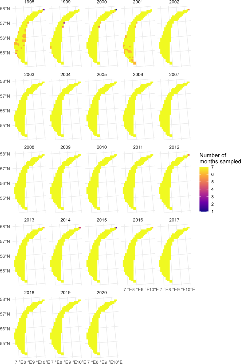
To illustrate the spatial and temporal distribution of in-situ and EO measurements, data were aggregated at a 10×10 km grid scale and visualized on maps showing the number of months each grid was sampled per year (Figure 7, Figure 8, Figure 9 for in-situ, and Figure 10, Figure 11, Figure 12 for EO).
In the CFR, not all years contain in-situ measurements; only a single grid near the coast was repeatedly sampled across years and throughout the growing season (Figure 7). In the KC, in-situ measurements are mainly located near the Danish coast, with one additional grid near the Swedish coast, these grids also show the most consistent sampling throughout the growing season (Figure 8). In the OC, only the northernmost grid was sampled throughout the growing season, with substantial variation in the number of sampling points per year and limited spatial coverage between 2005 and 2014 (Figure 9). In contrast, EO data provides high-resolution spatial and temporal coverage across all years and all areas (Figure 10, Figure 11, Figure 12).
| In-situ | EO | %In-situ | In-situ | EO | %In-situ | In-situ | EO | %In-situ | |
|---|---|---|---|---|---|---|---|---|---|
| 1998 | 7 | 270888 | 0,0026 | 49 | 415053 | 0,0118 | 73 | 597283 | 0,0122 |
| 1999 | 1 | 385688 | 0,0003 | 49 | 614801 | 0,0080 | 40 | 1078278 | 0,0037 |
| 2000 | 0 | 292744 | 0,0000 | 44 | 526614 | 0,0084 | 42 | 932049 | 0,0045 |
| 2001 | 0 | 313255 | 0,0000 | 45 | 603839 | 0,0075 | 42 | 1059945 | 0,0040 |
| 2002 | 7 | 456942 | 0,0015 | 50 | 912107 | 0,0055 | 43 | 1386105 | 0,0031 |
| 2003 | 11 | 712787 | 0,0015 | 60 | 1224233 | 0,0049 | 57 | 1970981 | 0,0029 |
| 2004 | 8 | 615032 | 0,0013 | 28 | 1296660 | 0,0022 | 57 | 1636097 | 0,0035 |
| 2005 | 60 | 614589 | 0,0098 | 26 | 1254693 | 0,0021 | 46 | 1898120 | 0,0024 |
| 2006 | 10 | 613570 | 0,0016 | 30 | 1171732 | 0,0026 | 38 | 1931795 | 0,0020 |
| 2007 | 0 | 547401 | 0,0000 | 38 | 1185808 | 0,0032 | 29 | 1893779 | 0,0015 |
| 2008 | 0 | 561864 | 0,0000 | 47 | 1316573 | 0,0036 | 21 | 1861476 | 0,0011 |
| 2009 | 1 | 590574 | 0,0002 | 36 | 1141516 | 0,0032 | 34 | 1896192 | 0,0018 |
| 2010 | 0 | 697759 | 0,0000 | 34 | 1076939 | 0,0032 | 27 | 1734009 | 0,0016 |
| 2011 | 0 | 565065 | 0,0000 | 29 | 1108461 | 0,0026 | 17 | 1539920 | 0,0011 |
| 2012 | 0 | 577974 | 0,0000 | 30 | 761390 | 0,0039 | 25 | 1695155 | 0,0015 |
| 2013 | 0 | 578220 | 0,0000 | 46 | 937487 | 0,0049 | 36 | 2175275 | 0,0017 |
| 2014 | 0 | 637876 | 0,0000 | 36 | 850056 | 0,0042 | 24 | 1928928 | 0,0012 |
| 2015 | 32 | 659810 | 0,0048 | 45 | 837279 | 0,0054 | 34 | 1757931 | 0,0019 |
| 2016 | 27 | 653190 | 0,0041 | 39 | 980776 | 0,0040 | 37 | 1967185 | 0,0019 |
| 2017 | 9 | 659264 | 0,0014 | 33 | 967052 | 0,0034 | 35 | 1795421 | 0,0019 |
| 2018 | 9 | 724620 | 0,0012 | 29 | 1184638 | 0,0024 | 94 | 2162929 | 0,0043 |
| 2019 | 10 | 659467 | 0,0015 | 42 | 1246141 | 0,0034 | 35 | 1762273 | 0,0020 |
| 2020 | 7 | 749603 | 0,0009 | 43 | 1451071 | 0,0030 | 29 | 2115286 | 0,0014 |
Figure 7. Distribution of in-situ measurements on a 10×10 km grid in the CFR assessment area per year from March until September. Colors indicate the number of months a grid cell was sampled during the growing season.
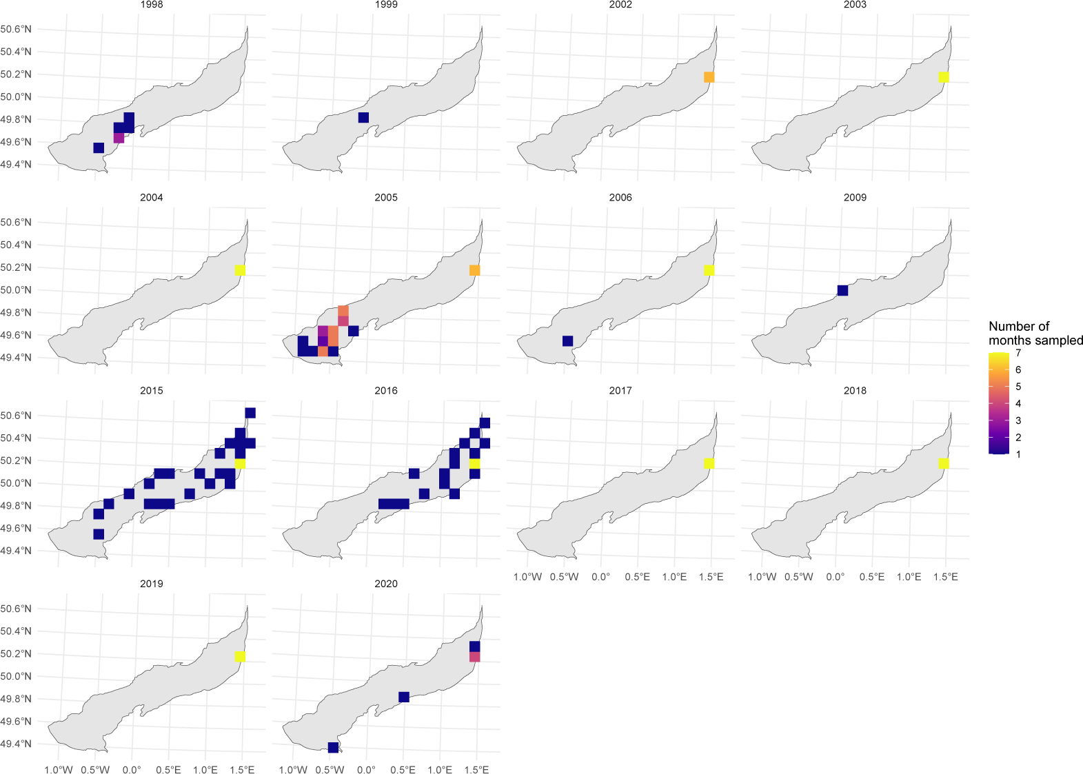
Figure 8. Distribution of in-situ measurements on a 10×10 km grid in the KC assessment area per year from March until September. Colors indicate the number of months a grid cell was sampled during the growing season.
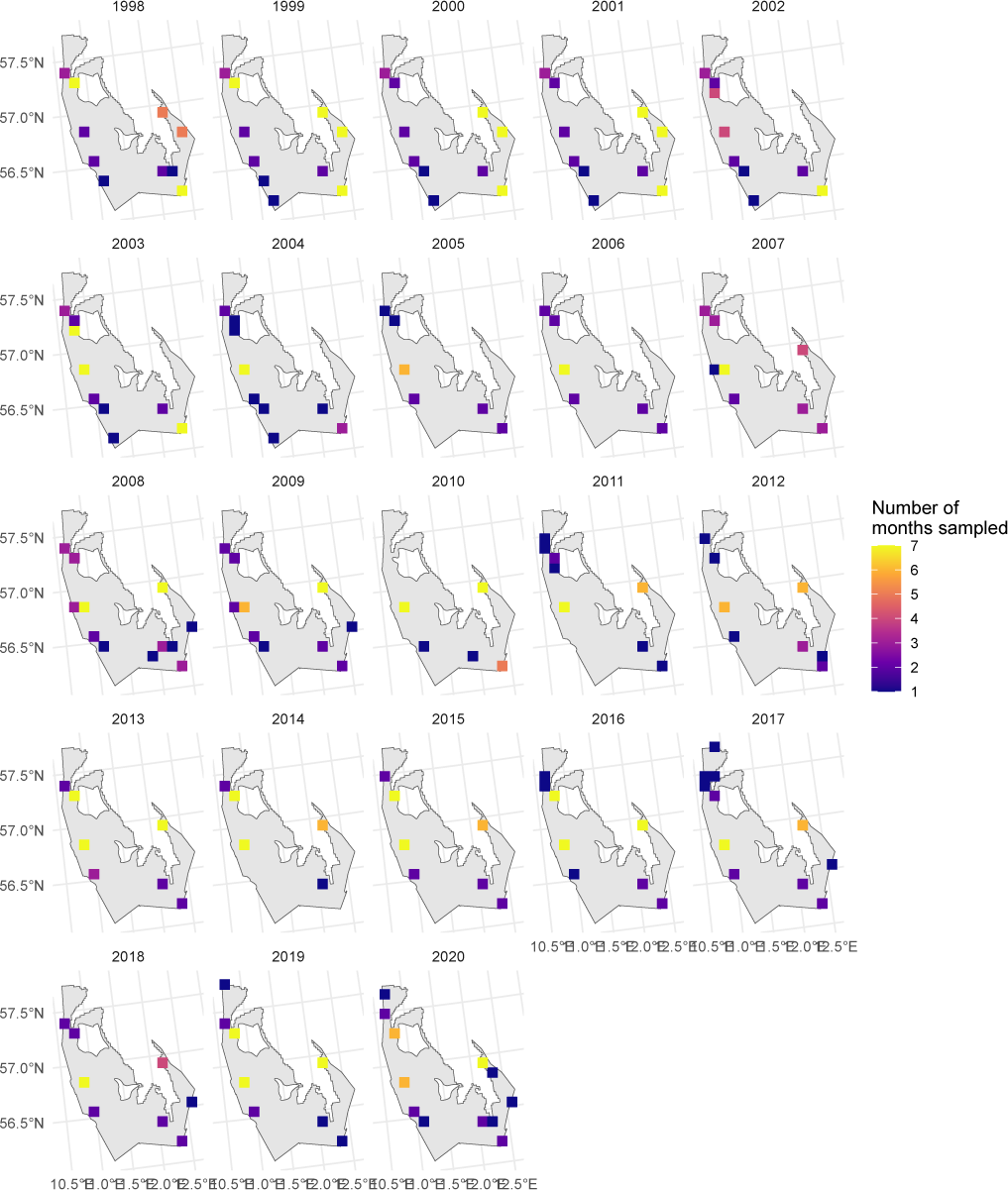
Figure 9. Distribution of in-situ measurements on a 10×10 km grid in the OC assessment area per year from March until September. Colors indicate the number of months a grid cell was sampled during the growing season.
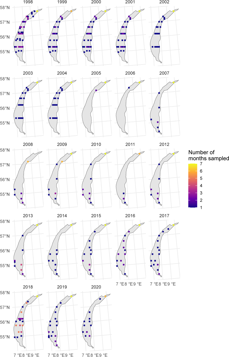
Figure 10. Distribution of EO measurements on a 10×10 km grid in the CFR assessment area per year from March until September. Colors indicate the number of months a grid cell was sampled during the growing season.
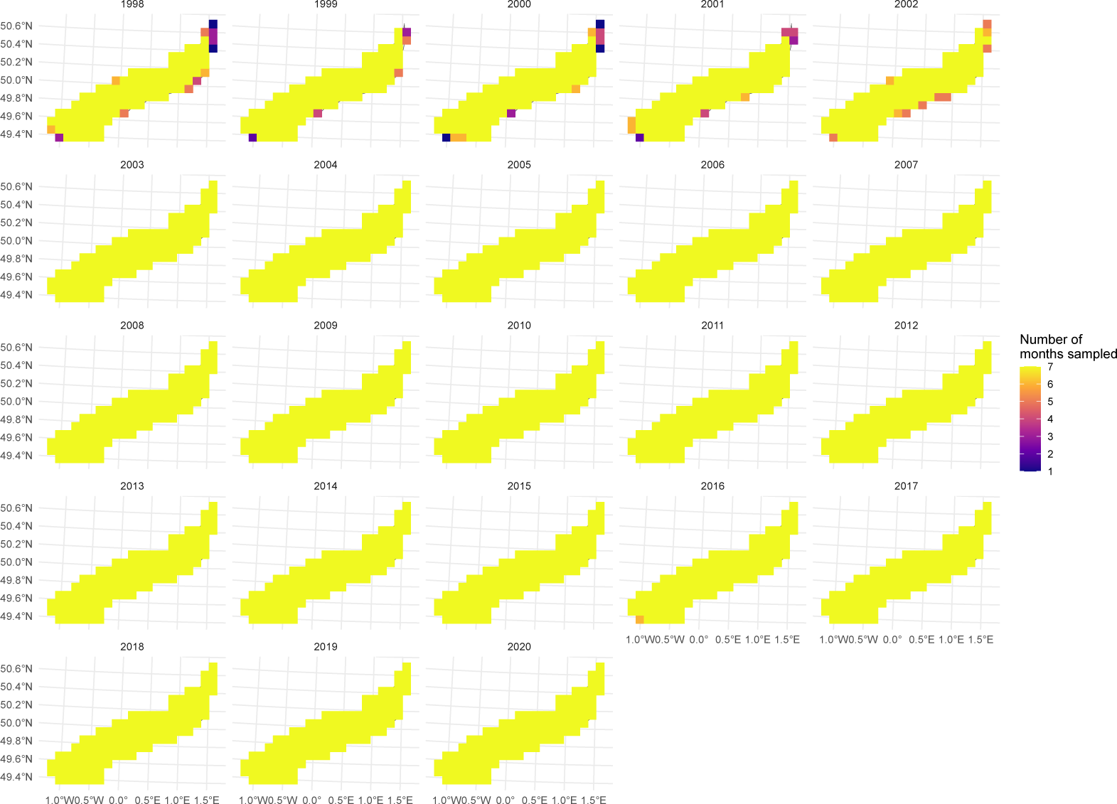
Figure 11. Distribution of EO measurements on a 10×10 km grid in the KC assessment area per year from March until September. Colors indicate the number of months a grid cell was sampled during the growing season.
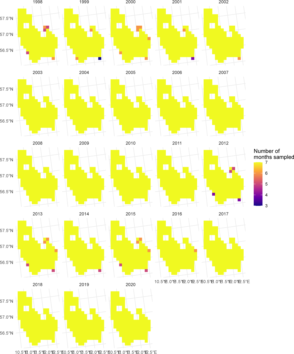
Figure 12. Distribution of EO measurements on a 10×10 km grid in the OC assessment area per year from March until September. Colors indicate the number of months a grid cell was sampled during the growing season.
5.2 Trends
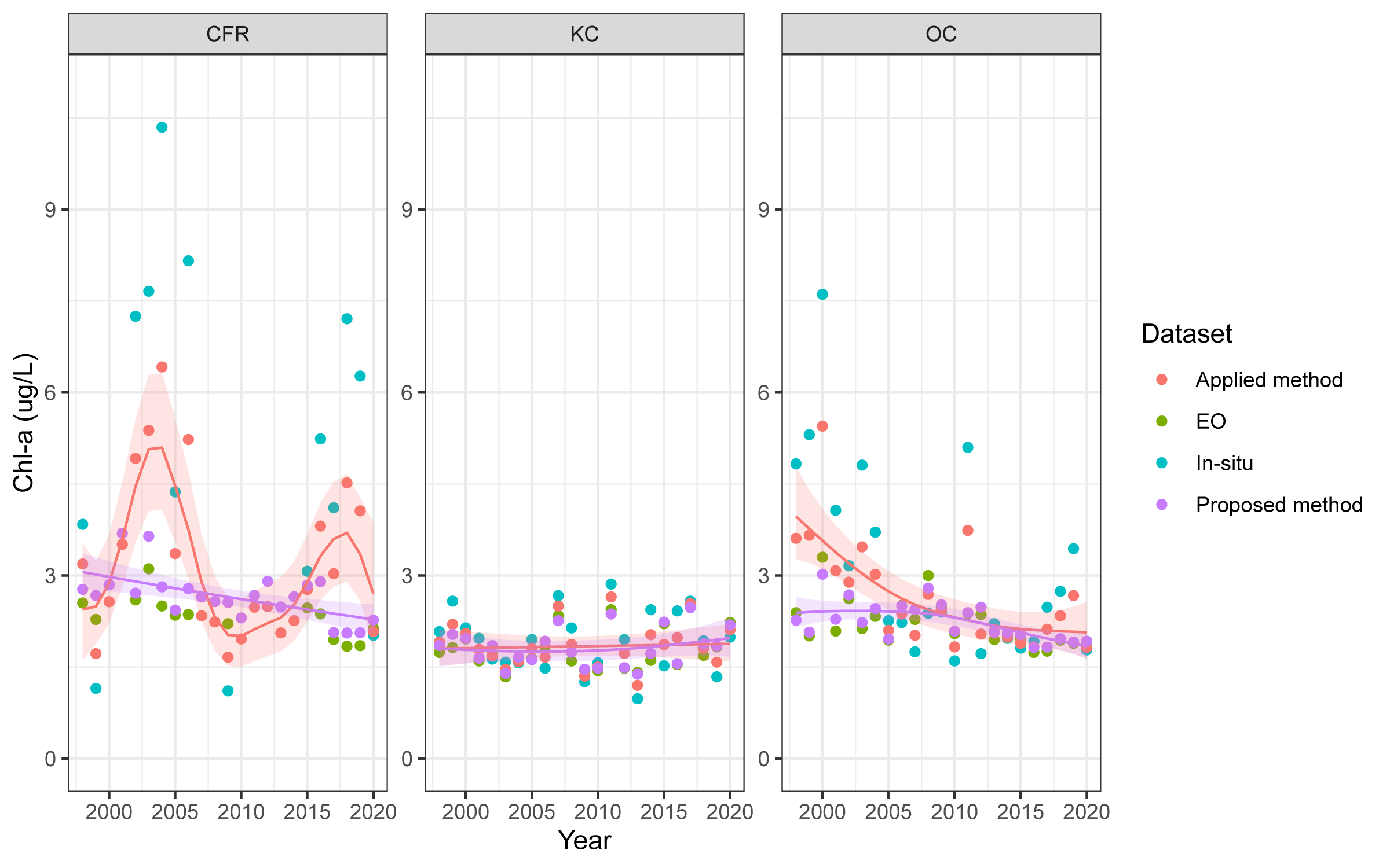
Differences in mean growing season chl-a concentrations between 1998-2020 were assessed for the different methods (Figure 13). The applied approach published on COMPEAT uses a weighted combination of in-situ and EO data (50:50). In contrast, the proposed method first aggregates data on a 10×10 km grid scale per month and year before calculating growing season means. This approach corrects for spatiotemporal sampling biases during the growing season and treats in-situ measurements as individual observations alongside EO data. A 10×10 km grid was chosen in the first aggregation step as the surface area of all three assessments areas was large enough (see section 4).
The two approaches produced differing trends calculated with Trendspotter5) in the CFR and OC.
In the CFR, the 50% weight of in-situ measurements resulted in considerably higher chl-a means in the applied method between 2002–2006 and 2016–2019 compared to the proposed method, with minimal overlap of the 95% confidence intervals over the entire period. In-situ chl-a concentrations during these periods were largely based on only one repeatedly measured sampling site close to the shore. Between 2007 and 2014, almost no in-situ measurements were available, causing the OSPAR chl-a means to exactly follow the EO data. Chl-a means calculated with the proposed method are slightly higher because of the first aggregation step.
In the OC, applying 50% weights to in-situ measurements resulted in higher chl-a means for the applied method between 1998 and 2005 compared to the proposed method, without overlap of the 95% confidence intervals. Although the in-situ sampling points were spatially fairly evenly distributed across the OC during that period, their temporal distribution was not: excluding the repeatedly measured northernmost site, 85% of samples were collected only in April and August, which may have introduced a temporal bias in in-situ chl-a concentrations.
In contrast, in the KC the trends derived from applied method and the proposed method were similar in both EO and in-situ datasets.
Figure 13. Chlorophyll-a growing season means between 1998-2020 for the OSPAR assessment areas CFR, KC and OC. Different colored points show the means according to the in-situ data (blue), EO data (green), and applying the proposed method (purple) or the applied method used by OSPAR (red). For the latter two, trendlines calculated with Trendspotter including a 95% confidence interval are also shown.
5.3 COMP4 assessment
The COMP4 assessment of the chl-a eutrophication status was repeated for the CFR, OC and KC OSPAR assessment areas using the proposed method and compared to the results published on COMPEAT (Table 5). The down-weighting of in-situ data according the confidence rating was not applied on COMPEAT, see annex I for the results in these assessment areas according to the agreed method (on average 70:30 weighting for EO to in-situ data in CFR; although no shifts in status occurred).
To determine the confidence ratings for each area, sample sizes corresponding to error ranges of 10% and 5% were calculated using the relative margin of error (MOE) (see section 4.4 of the previous report6)). For all three areas, the 10% threshold between ‘Low’ and ‘Moderate’ confidence corresponds to a sample size of approximately 50, while the 5% threshold between ‘Moderate’ and ‘High’ confidence corresponds to a sample size of approximately 220.
| Applied method | Proposed method | |||||||||
|---|---|---|---|---|---|---|---|---|---|---|
| Area | Period | TV | Chl-a (ug/L) | EQRS | Status | Confidence rating | Chl-a (ug/L) | EQRS | Status | Confidence rating |
| CFR | 2015-2020 | 2,8 | 3,4 | 0,49 | Moderate | High | 2,0 | 0,91 | High | High |
| KC | 2015-2020 | 1,2 | 2,0 | 0,25 | Poor | High | 2,0 | 0,21 | Poor | High |
| OC | 2015-2020 | 1,6 | 2,1 | 0,39 | Poor | High | 1,9 | 0,46 | Moderate | High |
Figure 14. EQRS for the OSPAR assessment area’s CFR, KC, and OC, between 2015-2020 as applied in COMP4 and according to the proposed method.
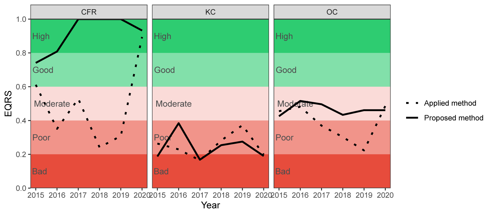
Using our proposed method, mean growing season chl-a concentrations were lower than those reported currently on COMPEAT for the CFR and OC (Table 5). This difference results from the reduced influence of in-situ data, which was more affected by extreme chl-a values due to its smaller sample size and sporadic sampling in these areas compared to the EO data (Figure 13). The reduced weighting of in-situ data leads to higher EQRS values and consequently a more positive eutrophication status: in the CFR, the status improved from Moderate to High, and in the OC from Poor to Moderate. Annual EQRS differences for COMP4 are shown in Figure 14, where EQRS values are generally higher under the proposed method, with status changes observed in several years for the CFR and OC assessment areas.
In contrast, in the KC assessment area, differences between mean chl-a concentrations from EO and in-situ data were less pronounced, resulting in comparable mean growing season values and identical eutrophication status as currently reported on COMPEAT and using the proposed method.
Confidence ratings were high in all three assessment areas using both the applied method and the proposed method.
5.4 Conclusion
The proposed method for assessing mean growing season chl-a concentrations and eutrophication status provides a more spatially and temporally balanced representation of conditions in the CFR, KC, and OC OSPAR assessment areas. By aggregating both in-situ and EO data on a 10×10 km grid scale per month and year, the novel approach corrects for biases caused by uneven sampling frequency and limited spatial coverage, particularly from the in-situ dataset.
In-situ data contributed only a very small fraction of the total measurements and were often concentrated in a few coastal grids, with several years lacking in-situ observations altogether. Consequently, the strong influence of extreme chl-a values in the applied 50:50 weighted approach led to higher mean chl-a concentrations in the CFR and OC compared to the proposed method. By reducing this disproportionate influence, the proposed method produced higher EQRS values and thus a more positive eutrophication status: the CFR improved from a Moderate to a High status, and the OC from a Poor to a Moderate status. In the KC, where in-situ and EO data were more consistent, results between the two approaches were largely comparable.
The application of objective confidence thresholds based on sample size further strengthens the transparency and reproducibility of the evaluation. Boundaries between confidence classes can be set based on the acceptable error range (here 10% and 5%).
Overall, the proposed method enhances the robustness of chl-a eutrophication assessments by providing a more objective and spatiotemporal representative integration of EO and in-situ observations. This approach can serve as a consistent and adaptable framework for future OSPAR assessments, improving comparability across regions and years.