Chlorophyll-a Trends in OSPAR Assessment Areas: Applying and Evaluating a New Statistical Approach
About this publication
This report expands on a newly proposed method for assessing chlorophyll-a (chl-a) concentrations and eutrophication status within the OSPAR framework. The method aggregates in-situ and Earth Observation (EO) data on a grid-month-year basis before calculating the growing season mean, with a confidence rating derived from the sample size for each grid. This approach aims to reduce biases introduced by limited and sporadic in-situ sampling, which often disproportionately influences chl-a concentrations. Compared to the applied method on COMPEAT, which equally weights in-situ and EO data, the proposed method leads to lower mean growing season chl-a concentrations and a higher Ecological Quality Ratio Scaled (EQRS), often resulting in improved eutrophication status. This difference is particularly evident in areas with limited in-situ data, such as small river plume assessment areas.
The report also examines the influence of grid resolution, used in the proposed method, on assessment outcomes, recommending a 5×5 km grid for areas smaller than 205 km2 and a 10×10 km grid for areas larger than 580 km2. A confidence rating system based on sample size further enhances the robustness of the assessment, providing a clearer understanding of the uncertainty involved.
The proposed method offers a transparent, objective, and spatiotemporally representative approach to eutrophication assessments, aligning with OSPAR’s goals for harmonized data aggregation. Its broader applicability across OSPAR assessment areas demonstrates its potential for improving future assessments and policy decisions related to marine eutrophication.
1. Introduction
Accurate knowledge of chlorophyll-a (chl-a) concentrations is essential for understanding primary production and evaluating eutrophication status in marine ecosystems. Within the OSPAR framework, chl-a serves as a key indicator for assessing eutrophication under the Common Procedure Eutrophication Assessment Tool (COMPEAT). In the previous Statistics Netherlands (CBS) report, the COMPEAT methodology used to assess chl-a concentrations in the OSPAR maritime area was evaluated, specifically focusing on OSPAR assessment areas such as the Southern North Sea (SNS), Meuse plume (MPM), and Rhine plume (RHPM)1) that (partly) overlap with Dutch waters. A newly developed method was proposed (henceforth referred to as the ‘proposed method’) to calculate growing season means and for determining confidence ratings, by first aggregating both in-situ and Earth Observation (EO) data on a grid basis, before assigning confidence ratings based on the sample size per grid. Under the COMPEAT approach currently applied by OSPAR (during the COMP4 assessment; henceforth referred to as the ‘applied method’), EO and in-situ data are combined with equal weighting (50:50), provided that in-situ data show a high confidence as otherwise they will be down-weighted, when calculating the growing season mean chl-a concentration per assessment area.
This report builds upon this proposed method and explores its implications in more detail by 1) revising a figure from the previous report to more accurately represent the temporal coverage of in-situ measurements and providing trends for the coastal OSPAR assessment areas that overlap with Dutch waters, 2) examining the method’s impact on the chl-a assessment for the three previously examined OSPAR assessment areas, 3) focusing on the smaller river plume OSPAR assessment areas to identify an optimal grid size that balances the reliability of growing season chl-a means with a high confidence rating, and 4) applying the method to additional OSPAR assessment areas that were not part of its initial development, to test its broader applicability and evaluate its influence on chl-a assessments.
2. Revision figures
2.1 Temporal coverage of in-situ measurements
The previous report illustrated the temporal coverage of in-situ measurements in the SNS assessment area by showing how many months each site was sampled each year, based on the exact coordinates of individual monitoring locations (Figure 1). The challenge with this visualization approach is that the temporal coverage might not align well with the sampling strategy used by some countries, most notably the United Kingdom, which follows a random sampling design rather than fixed monitoring stations. In such cases, multiple measurements may be taken within the same grid cell during a single growing season, even though no fixed location is sampled consistently over time.
To more accurately reflect the temporal coverage of in-situ sampling under such designs, Figure 1 should be revised to show the number of months sampled per grid cell per year, rather than per fixed site. This would better capture the actual sampling effort, particularly in areas where fixed locations are not used (Figure 2). This also aligns better with our improved method, in which growing season means are first aggregated on a grid basis.
Figure 1. Distribution of in-situ measurements in the SNS assessment area per year from March until September. Colors indicate the number of months a site was sampled during the growing season.
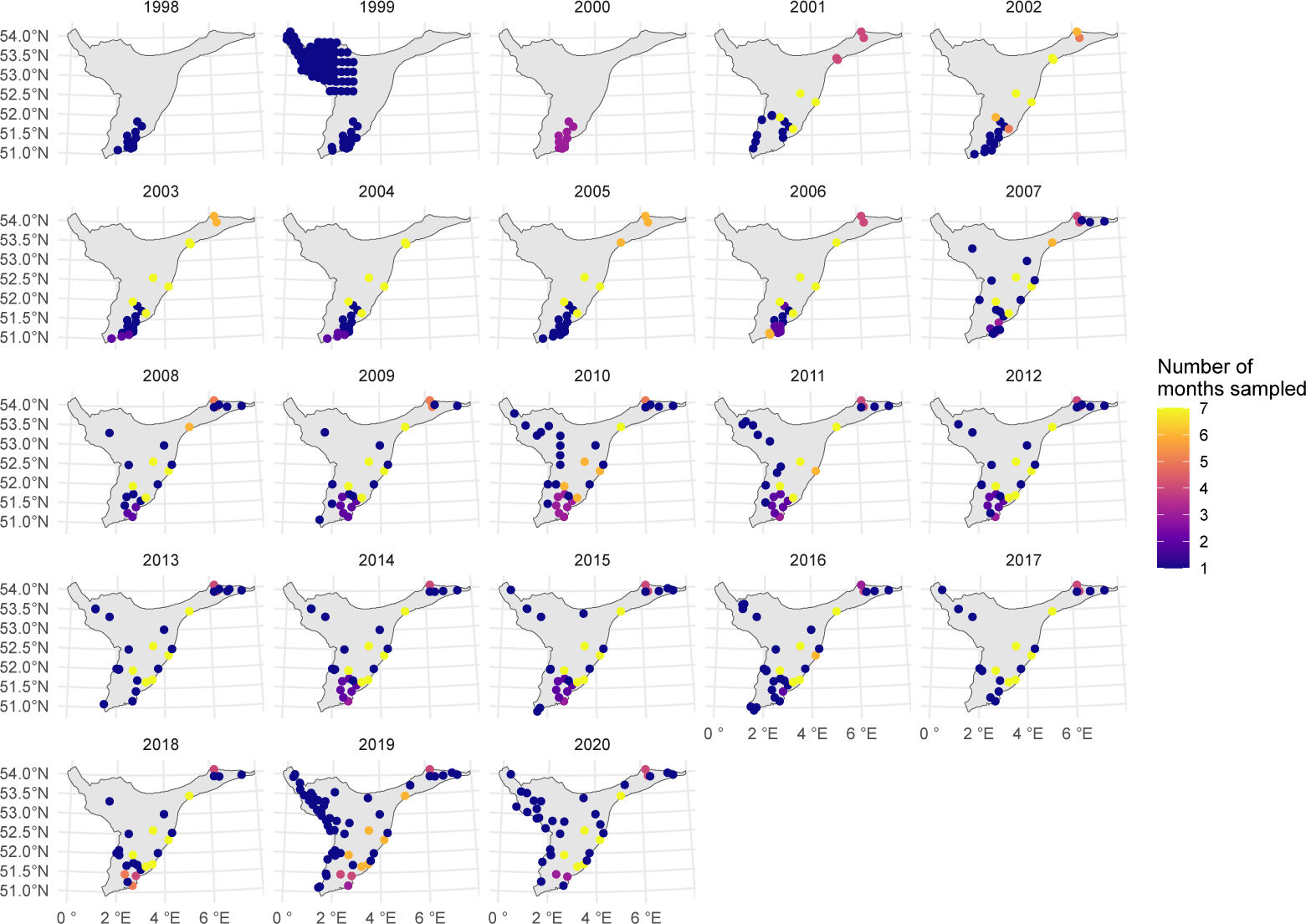
Figure 2. Revision of figure 1 from the previous report, showing the distribution of in-situ measurements on a 25×25 km grid in the SNS assessment area per year from March until September. Colors indicate the number of months a grid cell was sampled during the growing season.
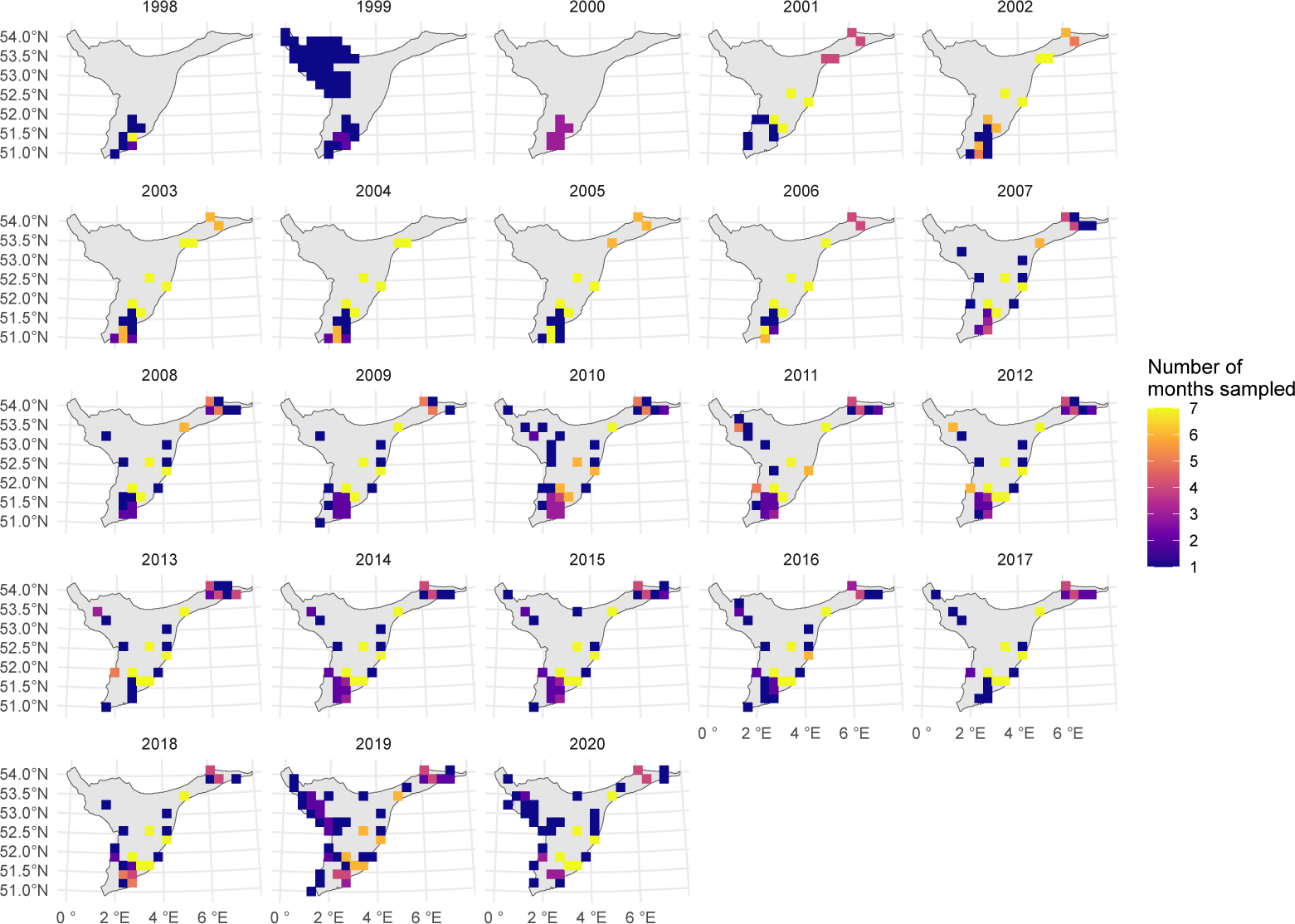
Figure 1 and 2 show that the temporal coverage of in-situ measurements does not differ substantially when comparing grid cell-based data to exact location data. In Figure 1, 784 points are shown using exact coordinates, compared to 518 points using the 25×25 km grid approach (Figure 2). The number of points with repeated measurements is slightly higher in the grid-based version (269) than in the exact location version (252). Similarly, the average number of months sampled per point is marginally higher when using grid cells, with 3 months compared to 2.3 months for exact locations. However, only over half of all the grid cells at a 25×25 km resolution are sampled, when considering just in-situ data. In years when more locations were sampled off the British coast, most measurements were concentrated in one (July 1999) or two months (July/August 2019 and July/September 2020) within the growing season, rather than being distributed across multiple months. Consequently, only minor differences in temporal coverage are expected between the two figures.
2.2 Conclusion
Although the UK employs a random sampling design, measurements do not always occur in different months each year. As a result, a different visualization approach does not greatly improve the overall temporal coverage of in-situ data.
2.3 Trends RHPM and MPM
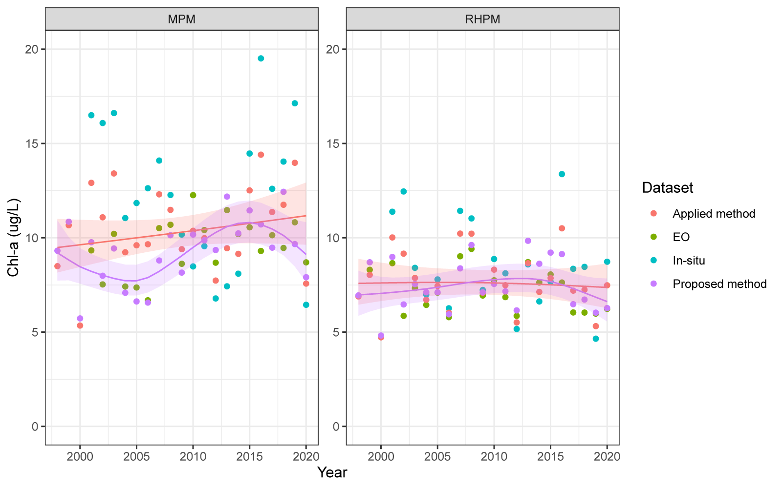
Trends in mean growing season chl-a concentrations between 1998-2020 were assessed for the applied method and the proposed method, but only for the SNS OSPAR assessment area in the previous report (see section 4.3)1). Figure 3 presents these trends, calculated with Trendspotter2), also for the MPM and RHPM areas. Trendspotter is a method to estimate flexible trendlines for time series data. The applied approach uses a weighted combination of in-situ and EO data (50:50). In contrast, the proposed method first aggregates data on a 10×10 km grid scale per month and year before calculating growing season means. This approach corrects for spatiotemporal sampling biases during the growing season and treats in-situ measurements as individual observations alongside EO data.
In the MPM, both methods reveal distinct trends (although with substantial overlap of 95% confidence intervals): while the applied method indicates a steady increase, the proposed method shows a peak around 2015 followed by a decline in recent years. Over time, in-situ chl-a concentrations ranged from 6.8 until 19.5 µg/L, while EO chl-a concentrations ranged from 6.7 until 12.3 µg/L. In-situ data in this assessment area is also only based on one sampling site that is sampled each month during the growing season.
In the RHPM, the trends are more similar, though the post-2015 decrease is more pronounced in the proposed method. Over time, in-situ chl-a concentrations ranged from 4.7 until 13.4 µg/L, while EO chl-a concentrations ranged from 4.7 until 9.4 µg/L. In-situ data in the RHPM is based on three sampling site that are sampled each month during the growing season.
Figure 3. Chlorophyll-a growing season means between 1998-2020 for the OSPAR assessment areas MPM and RHPM. Different colored points show the means according to the in-situ data (blue), EO data (green), and applying the proposed method (purple) or the method applied by OSPAR (red). For the latter two, trendlines calculated with Trendspotter including a 95% confidence interval are also shown.
2.4 Conclusion
Subtle differences are observed in the temporal patterns between the proposed grid-based method and the applied approach used by OSPAR for calculating growing season mean chl-a in the MPM and RHPM assessment areas, although these differences are less pronounced than those found in the previous report for the SNS assessment area.
3. COMP4 assessment
In the OSPAR Common Procedure Eutrophication Assessment Tool (COMPEAT), the eutrophication status for each indicator, including chl-a, is classified on a scale from ‘Bad’ to ‘High3). This classification is based on indicator-specific thresholds defined for each OSPAR assessment area and scaled using the Ecological Quality Ratio Scaled (EQRS) approach4). Assessment results are reported for the growing season (March to September) and for defined assessment periods, spanning six years.
The fourth application of the Common Procedure (COMP4) covered the period 2015–2020. In this chapter, we repeated the COMP4 assessment for the SNS, MPM, and RHPM assessment areas using the newly proposed method, to evaluate whether it leads to different classification outcomes.
In Table 1, an overview of the results for the COMP4 per assessment area (including threshold value; TV, and differences in confidence rating) is given by comparing the assessment applied by OSPAR, weighting EO and in-situ chl-a seasonal means equally, and the improved method, which first aggregates EO and in-situ chl-a data on a 10×10 km scale per month and year before calculating growing season means and confidence ratings. The down-weighting of in-situ data according the confidence rating was not applied on COMPEAT, see annex I for the results in these assessment areas according to the agreed method (70:30 weighting for EO to in-situ data in MPM; although no shifts in status occurred).
| Applied method | Proposed method | |||||||||
|---|---|---|---|---|---|---|---|---|---|---|
| Area | Period | TV | Chl-a (ug/L) | EQRS | Status | Confidence rating | Chl-a (ug/L) | EQRS | Status | Confidence rating |
| MPM | 2015-2020 | 8 | 11,9 | 0,32 | Poor | High | 10,3 | 0,39 | Poor* | High* |
| RHPM | 2015-2020 | 6,8 | 7,6 | 0,53 | Moderate | High | 7,3 | 0,53 | Moderate | Moderate |
| SNS | 2015-2020 | 3,8 | 3,3 | 0,74 | Good | High | 3,0 | 0,83 | High | High |
| *See chapter 4 | ||||||||||
In the proposed method, mean growing season chl-a concentrations are generally lower than those reported by the applied method. This is likely due to the reduced influence of in-situ data, which tend to be more affected by extreme chl-a values because of the smaller sample size and more sporadic sampling, compared to the EO data. Due to the large amount of data, satellite data therefore exhibits a smoothing effect across the grid cells for the assessment area compared to the sporadic in-situ data, which can randomly capture algal blooms. For this reason, it is necessary to review and possibly adjust the associated chl-a threshold values.
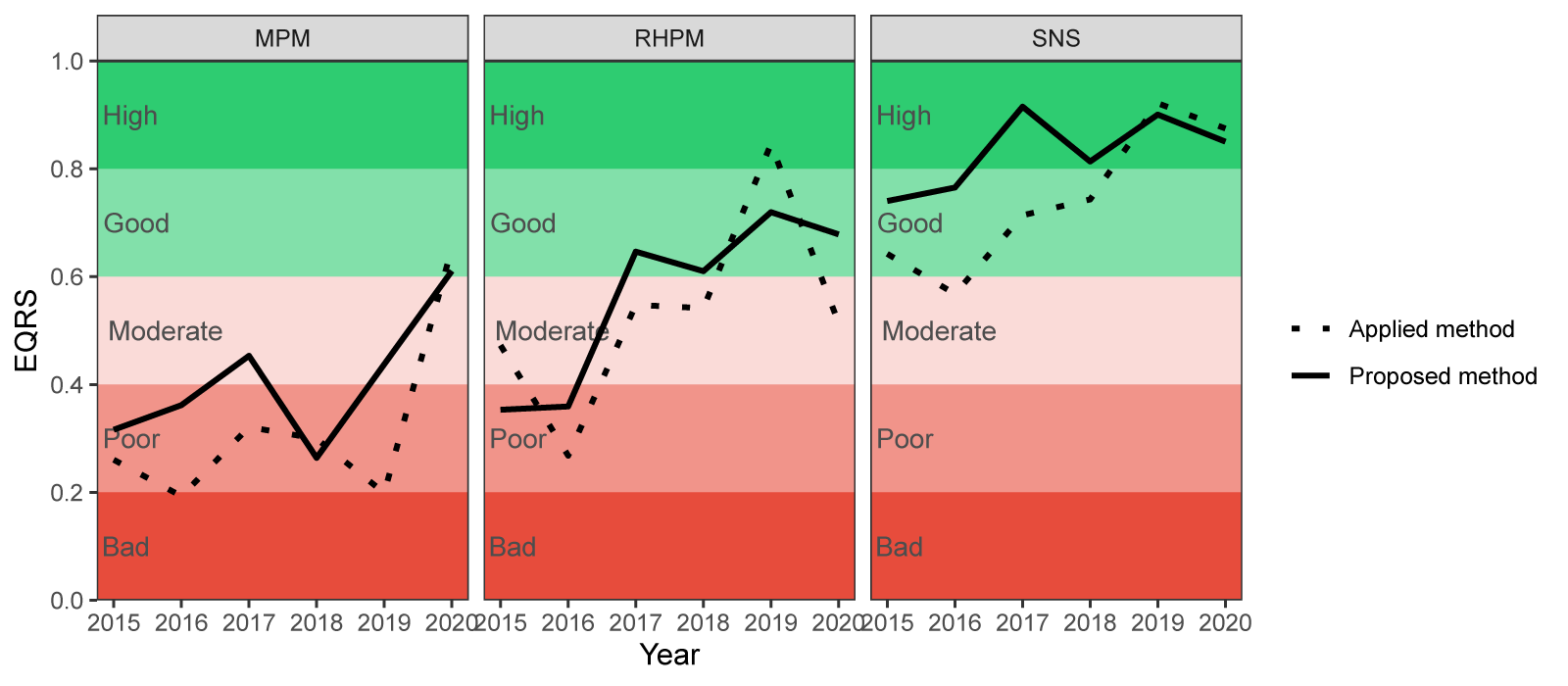
This reduced influence of in-situ data leads to a higher EQRS and a more positive status. For example, the status for SNS increased from Good to High. Differences in EQRS per year for COMP4 are shown in Figure 4. As mentioned before, EQRS values are generally higher in the proposed method, show less variation between the years, and have a different status in some years.
Figure 4. EQRS per OSPAR assessment area between 2015-2020 as applied in COMP4 and according to the proposed method.
In addition to differences in mean growing season chl-a concentrations, a newly proposed method for inferring confidence rating based on sample size was also introduced. The current method used by OSPAR for assigning a confidence rating is the same for in-situ and EO data, and the criteria lack a formal statistical foundation (for details, see Annex 13 of the OSPAR eutrophication status assessment procedure)4). The novel method uses the sample size from each year–month–grid combination, which is then aggregated to derive an overall confidence rating for the chl-a growing season mean each year. Confidence classes are derived using the relative margin of error (MOE; which quantifies the amount of random sampling error, for details see section 4.4 of the previous report)1). The classes are defined as follows: ‘Low’ confidence corresponds to an error range > 10% and a sample size < 50 or 60 (SNS or coastal zone), ‘Moderate’ to an error range between 10% and 5% and sample sizes between 50 and 200 or 60 and 260 (SNS or coastal zone), and ‘High’ to an error range < 5% and a sample size > 200 or 260 (SNS or coastal zone). Sample sizes required to reach a certain error range were determined per assessment area following the approach from the previous report, as each area exhibits different chl-a concentrations and fluctuation patterns.
It should be noted that the error ranges of 10% and 5% were coined in the previous report as more objective boundaries for determining the confidence ratings, but these can be adjusted to the accepted error range, which is up to policy, and can also be area specific.
This leads to differences in the overall confidence rating for COMP4, where RHPM scored Moderate instead of High based on the stricter, but more statistically founded method. This was expected, as the criteria for determining the confidence rating used in the applied method were based on the in-situ data alone.
3.1 Conclusion
Applying the proposed method to the COMP4 assessment for the SNS, MPM, and RHPM areas resulted in generally lower mean growing season chl-a concentrations compared to the results published on COMPEAT. This difference is mainly due to the reduced influence of in-situ data, which are more prone to extreme values because of their limited and irregular sampling frequency. As a result, the proposed method produced higher EQRS values and, in some cases, a more favorable eutrophication status (e.g., from Good to High in the SNS).
The proposed approach for deriving confidence ratings, which explicitly accounts for sample size and statistical uncertainty, led to more differentiated and statistically grounded confidence classes. While this method resulted in lower confidence ratings for some assessment areas (e.g., RHPM), it provides a more robust and transparent basis for interpreting chl-a assessment outcomes within COMPEAT.
4. Optimal grid resolution for river plumes
In the previous report, we primarily focused on the SNS assessment area to determine the optimal grid resolution for calculating growing season means and concomitant confidence ratings. Here, we revisit the smaller assessment areas, i.e. river plumes, along the Dutch coast in more detail to determine whether aggregation of chl-a on a 10×10 km scale is indeed optimal for the assessment procedure. We applied the proposed assessment method for the RHPM, MPM, SCHPM1 (Scheldt plume 1), and SCHPM2 (Scheldt plume 2) assessment areas, using three different grid resolutions, 10×10, 5×5 and 2×2 km, and evaluated the results.
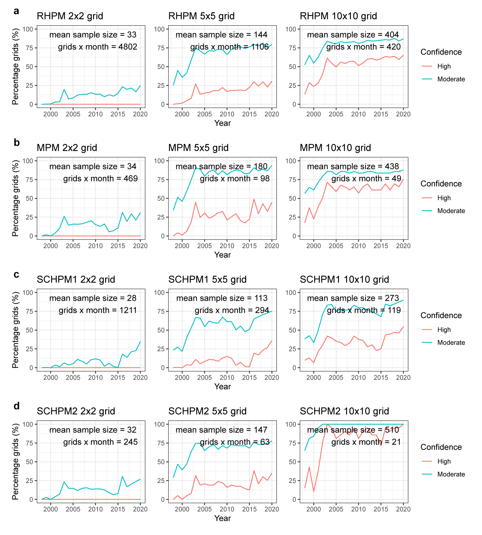
As grid size increases, more chl-a measurements are included in each year-month-grid aggregation. This leads to a general increase in confidence ratings, as a higher proportion of grid cells meets the thresholds for moderate (>60 samples) and high (>260 samples) confidence (Figure 5). Additionally, advances in satellite sensors and data processing algorithms have led to a higher proportion of grid cells reaching these confidence thresholds over the course of the study period.
The downside of using a coarser grid is that it reduces the number of distinct spatial units within an assessment area, thereby lowering the total number of grid-month combinations available for calculating growing season means (Figure 5). The number of months per growing season (seven) remains the same across all grid resolutions, but finer grids provide a more spatially detailed representation of the assessment area. This trade-off between spatial resolution and confidence should also be considered when selecting the appropriate grid size for each assessment area.
The COMP4 assessment was repeated for the four assessment areas at varying spatial grid resolutions (Table 2), using area-specific threshold values (TVs). Mean growing season chl-a concentrations were generally consistent across grid resolutions, with the largest observed difference being 0.6 µg L⁻¹ between the 5×5 km and 10×10 km grids in the MPM area. This difference translated into a 0.04 change in EQRS.
Although these differences appear minor, they can still substantially influence the assigned eutrophication status because the method does not account for uncertainty. For example, both MPM and SCHPM2 shifted from Moderate to Poor status when moving from the 5×5 km to the 10×10 km grid. In the proposed method, the confidence rating (Moderate for 5×5 km and High for 10×10 km) reflects the uncertainty range around the mean. For MPM, the uncertainty was between 0.49 and 0.97 µg L⁻¹ at 5×5 km, and below 0.52 µg L⁻¹ at 10×10 km. For SCHPM2, uncertainty ranged from 0.56 to 1.11 µg L⁻¹ at 5×5 km and was below 0.58 µg L⁻¹ at 10×10 km. When this uncertainty is incorporated into the assessment, all grid resolutions for these areas yield the same eutrophication status, on the boundary between Moderate and Poor.
However, coarser grids reduce spatial detail, potentially masking local variation or ecologically relevant gradients. Both SCHPM2 and MPM are relatively small areas (95 km² and 205 km², respectively), corresponding to only 3–7 grid cells at 10×10 km resolution. Few formal guidelines exist on the minimum number of grid cells required to capture local variability meaningfully, as this depends on the spatial homogeneity of the area and the environmental parameter assessed.
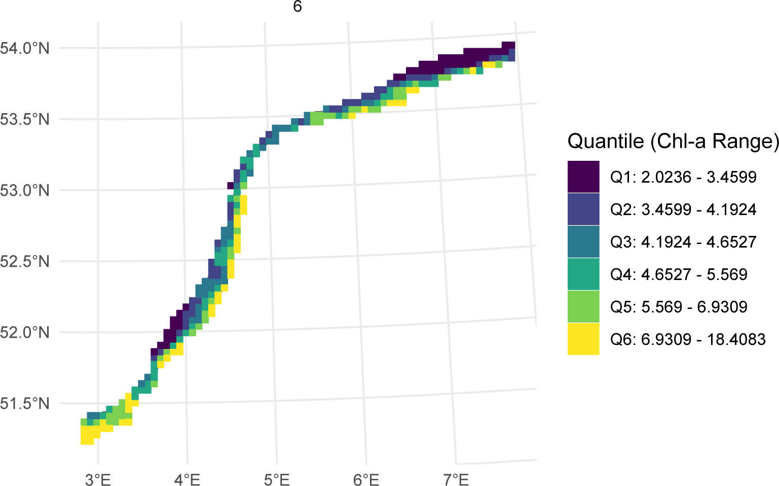
The OSPAR assessment areas were delineated to represent relatively homogeneous regions, implying broadly similar chl-a concentrations within each. Nevertheless, spatial gradients can still occur, as illustrated in Figure 6, which shows chl-a distribution across the Dutch river plume assessment areas in June 2020.
Although such gradients are not explicitly used in this assessment, setting a minimum threshold for the number of grid cells per assessment area, on which to base the growing-season mean, could be advisable and is ultimately a policy decision. For smaller areas such as MPM and SCHPM2, a finer grid resolution (5×5 km) may be preferable, provided that at least a Moderate confidence rating can be achieved. This approach maintains a balance between statistical reliability and spatial resolution.
Figure 5. Percentage of grids in the a) RHPM, b) MPM, c) SCHPM1, and d) SCHPM2 assessment areas with a confidence rating of at least High (> 260 measurements) or at least Moderate (> 60 measurements) from 1998 until 2020 for three different grid resolutions. In the graphs, the mean sample size per year-month-grid combination is indicated, as well as the maximum number of grid-month combinations per growing season.
| Area | Period | Grid resolution (km) | TV | Chl-a (ug/L) | EQRS | Status | Confidence rating |
|---|---|---|---|---|---|---|---|
| MPM | 2015-2020 | 2x2 | 8 | 10,0 | 0,41 | Moderate | Low |
| MPM | 2015-2020 | 5x5 | 8 | 9,7 | 0,43 | Moderate | Moderate |
| MPM | 2015-2020 | 10x10 | 8 | 10,3 | 0,39 | Poor | High |
| RHPM | 2015-2020 | 2x2 | 6,8 | 7,0 | 0,57 | Moderate | Low |
| RHPM | 2015-2020 | 5x5 | 6,8 | 7,2 | 0,55 | Moderate | Moderate |
| RHPM | 2015-2020 | 10x10 | 6,8 | 7,3 | 0,53 | Moderate | Moderate |
| SCHPM1 | 2015-2020 | 2x2 | 5 | 12,4 | 0,14 | Bad | Low |
| SCHPM1 | 2015-2020 | 5x5 | 5 | 12,4 | 0,14 | Bad | Moderate |
| SCHPM1 | 2015-2020 | 10x10 | 5 | 12,1 | 0,14 | Bad | Moderate |
| SCHPM2 | 2015-2020 | 2x2 | 8,9 | 11,1 | 0,41 | Moderate | Low |
| SCHPM2 | 2015-2020 | 5x5 | 8,9 | 11,1 | 0,41 | Moderate | Moderate |
| SCHPM2 | 2015-2020 | 10x10 | 8,9 | 11,5 | 0,39 | Poor | High |
Figure 6. Quantile chlorophyll-a concentrations (μg L<sup>-1</sup>) summarized on a 5×5 km scale in the RHPM, MPM, SCHPM1, and SCHPM2 assessment area’s in June 2020.
If these changes are applied to Table 1 from Section 3, the eutrophication status and the confidence rating for MPM will shift from Poor to Moderate and High to Moderate, respectively (Table 3). Notably, the mean growing season chl-a concentration under the proposed method is lower than the value reported by the applied method on COMPEAT. This difference is primarily due to the disproportionate influence of the in-situ data in this assessment area in the reported OSPAR method. Only one in-situ monitoring site is sampled throughout all months of the growing season, yet it is weighted equally (50%) relative to the EO data, which leads to an overrepresentation of that single in-situ signal in the final result.
The results for SCHPM1 and SCHPM2 under the proposed method are largely consistent with those reported on COMPEAT. For SCHPM2, no in-situ monitoring sites are present, so both the applied method and the proposed method rely solely on EO data. SCHPM1 has a single in-situ monitoring site, similar to MPM; in this case, however, the in-situ values align more closely with the mean chl-a concentrations based on EO data and weighting them equally does not lead to a different eutrophication status.
| Applied method | Proposed method | |||||||||
|---|---|---|---|---|---|---|---|---|---|---|
| Area | Period | TV | Chl-a (ug/L) | EQRS | Status | Confidence rating | Chl-a (ug/L) | EQRS | Status | Confidence rating |
| MPM | 2015-2020 | 8 | 11,9 | 0,32 | Poor | High | 9,7 | 0,43 | Moderate | Moderate |
| SCHPM2 | 2015-2020 | 8,9 | 11,0 | 0,43 | Moderate | High | 11,1 | 0,41 | Moderate | Moderate |
| SCHPM1 | 2015-2020 | 5 | 12,2 | 0,15 | Bad | High | 12,1 | 0,14 | Bad | Moderate |
| RHPM | 2015-2020 | 6,8 | 7,6 | 0,53 | Moderate | High | 7,3 | 0,53 | Moderate | Moderate |
| SNS | 2015-2020 | 3,8 | 3,3 | 0,74 | Good | High | 3,0 | 0,83 | High | High |
4.1 Conclusion
The assessment of smaller Dutch OSPAR areas using different spatial grid resolutions showed that mean growing-season chl-a concentrations and EQRS values were largely consistent across grid sizes. Although coarser grids (10×10 km) increased statistical confidence by incorporating more samples per cell, they also reduced spatial detail, as the mean was based on fewer spatial grids per assessment area. In the smallest areas, such as MPM and SCHPM2, growing-season means were derived from only 3 – 7 grid cells in the 10×10 layout.
Nevertheless, the overall differences in mean chl-a concentrations and EQRS values between grid resolutions were minimal, suggesting that all tested grid sizes yield comparable assessment outcomes when uncertainty around the mean is considered. For small river plumes, a finer grid resolution (5×5 km) may still be preferred, provided that at least a Moderate confidence rating can be achieved, as it better preserves spatial gradients while maintaining sufficient statistical reliability.
5. Other assessment areas
The proposed method was developed using OSPAR assessment areas that overlap with Dutch waters. In this chapter, we explore how in-situ and EO data relate to one another in three other regions: the Outer Coastal DEDK (OC), the Kattegat Coastal (KC), and the Coastal French Channel (CFR). Both the OC and KC show a highly variable distribution of chl-a, with limited temporal and spatial coverage. These areas also have a poor environmental status (EQRS), making it essential to closely track future trends and potential improvements. The proposed method could offer a more accurate estimate of the true chl-a concentrations. In the CFR, a higher density of in-situ measurements near the coast may introduce a bias in overall chl-a, and applying the new method may also bring the results closer to the actual chl-a values.
5.1 Distribution in-situ and EO data
Table 4 presents the number of in-situ and EO measurements per year during the growing season for the CFR, KC, and OC, along with the percentage of in-situ measurements relative to the total. On average, only 0.0014%, 0.0045%, and 0.0027% of all growing season measurements are in-situ in the CFR, KC, and OC, respectively.
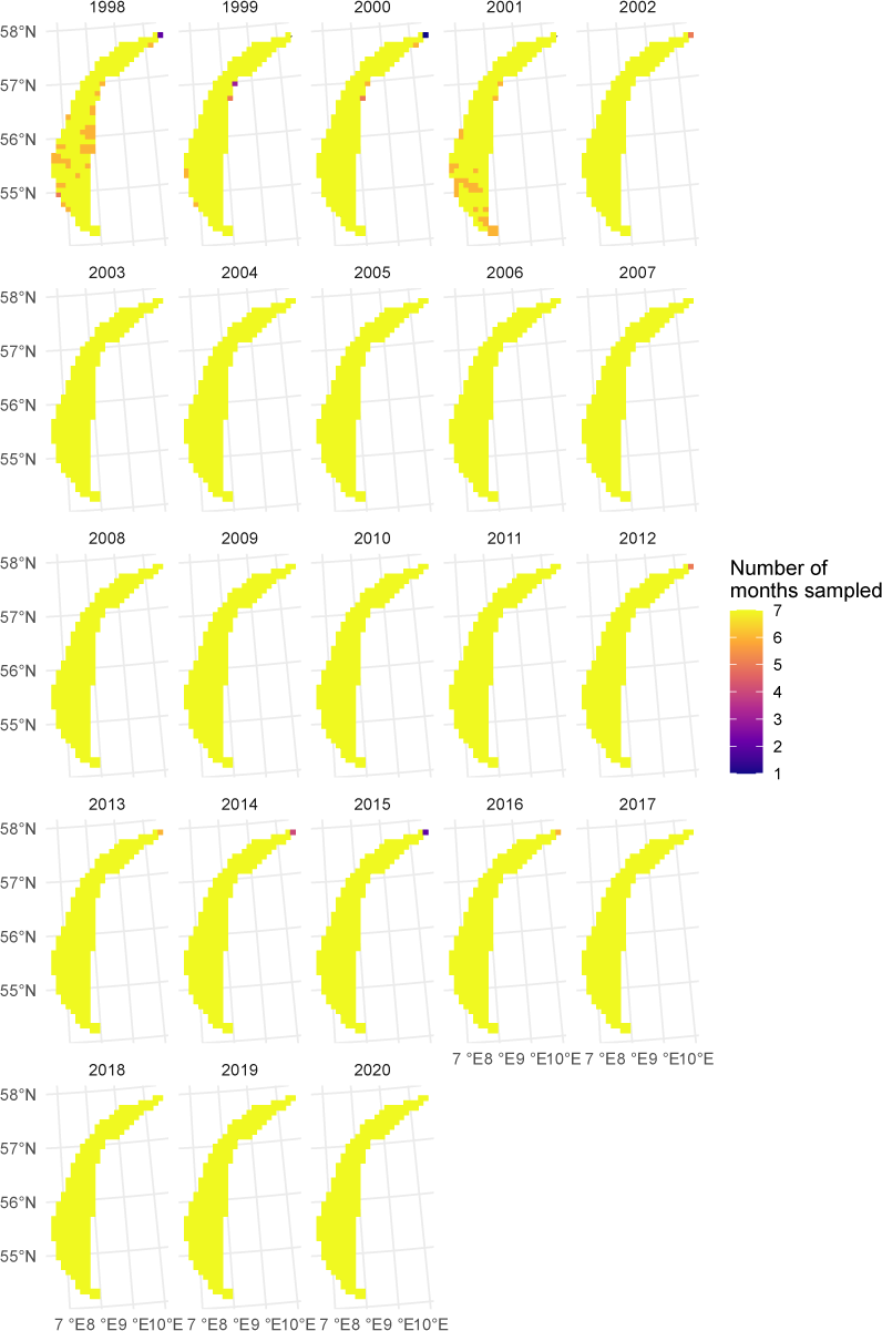
To illustrate the spatial and temporal distribution of in-situ and EO measurements, data were aggregated at a 10×10 km grid scale and visualized on maps showing the number of months each grid was sampled per year (Figure 7, Figure 8, Figure 9 for in-situ, and Figure 10, Figure 11, Figure 12 for EO).
In the CFR, not all years contain in-situ measurements; only a single grid near the coast was repeatedly sampled across years and throughout the growing season (Figure 7). In the KC, in-situ measurements are mainly located near the Danish coast, with one additional grid near the Swedish coast, these grids also show the most consistent sampling throughout the growing season (Figure 8). In the OC, only the northernmost grid was sampled throughout the growing season, with substantial variation in the number of sampling points per year and limited spatial coverage between 2005 and 2014 (Figure 9). In contrast, EO data provides high-resolution spatial and temporal coverage across all years and all areas (Figure 10, Figure 11, Figure 12).
| In-situ | EO | %In-situ | In-situ | EO | %In-situ | In-situ | EO | %In-situ | |
|---|---|---|---|---|---|---|---|---|---|
| 1998 | 7 | 270888 | 0,0026 | 49 | 415053 | 0,0118 | 73 | 597283 | 0,0122 |
| 1999 | 1 | 385688 | 0,0003 | 49 | 614801 | 0,0080 | 40 | 1078278 | 0,0037 |
| 2000 | 0 | 292744 | 0,0000 | 44 | 526614 | 0,0084 | 42 | 932049 | 0,0045 |
| 2001 | 0 | 313255 | 0,0000 | 45 | 603839 | 0,0075 | 42 | 1059945 | 0,0040 |
| 2002 | 7 | 456942 | 0,0015 | 50 | 912107 | 0,0055 | 43 | 1386105 | 0,0031 |
| 2003 | 11 | 712787 | 0,0015 | 60 | 1224233 | 0,0049 | 57 | 1970981 | 0,0029 |
| 2004 | 8 | 615032 | 0,0013 | 28 | 1296660 | 0,0022 | 57 | 1636097 | 0,0035 |
| 2005 | 60 | 614589 | 0,0098 | 26 | 1254693 | 0,0021 | 46 | 1898120 | 0,0024 |
| 2006 | 10 | 613570 | 0,0016 | 30 | 1171732 | 0,0026 | 38 | 1931795 | 0,0020 |
| 2007 | 0 | 547401 | 0,0000 | 38 | 1185808 | 0,0032 | 29 | 1893779 | 0,0015 |
| 2008 | 0 | 561864 | 0,0000 | 47 | 1316573 | 0,0036 | 21 | 1861476 | 0,0011 |
| 2009 | 1 | 590574 | 0,0002 | 36 | 1141516 | 0,0032 | 34 | 1896192 | 0,0018 |
| 2010 | 0 | 697759 | 0,0000 | 34 | 1076939 | 0,0032 | 27 | 1734009 | 0,0016 |
| 2011 | 0 | 565065 | 0,0000 | 29 | 1108461 | 0,0026 | 17 | 1539920 | 0,0011 |
| 2012 | 0 | 577974 | 0,0000 | 30 | 761390 | 0,0039 | 25 | 1695155 | 0,0015 |
| 2013 | 0 | 578220 | 0,0000 | 46 | 937487 | 0,0049 | 36 | 2175275 | 0,0017 |
| 2014 | 0 | 637876 | 0,0000 | 36 | 850056 | 0,0042 | 24 | 1928928 | 0,0012 |
| 2015 | 32 | 659810 | 0,0048 | 45 | 837279 | 0,0054 | 34 | 1757931 | 0,0019 |
| 2016 | 27 | 653190 | 0,0041 | 39 | 980776 | 0,0040 | 37 | 1967185 | 0,0019 |
| 2017 | 9 | 659264 | 0,0014 | 33 | 967052 | 0,0034 | 35 | 1795421 | 0,0019 |
| 2018 | 9 | 724620 | 0,0012 | 29 | 1184638 | 0,0024 | 94 | 2162929 | 0,0043 |
| 2019 | 10 | 659467 | 0,0015 | 42 | 1246141 | 0,0034 | 35 | 1762273 | 0,0020 |
| 2020 | 7 | 749603 | 0,0009 | 43 | 1451071 | 0,0030 | 29 | 2115286 | 0,0014 |
Figure 7. Distribution of in-situ measurements on a 10×10 km grid in the CFR assessment area per year from March until September. Colors indicate the number of months a grid cell was sampled during the growing season.
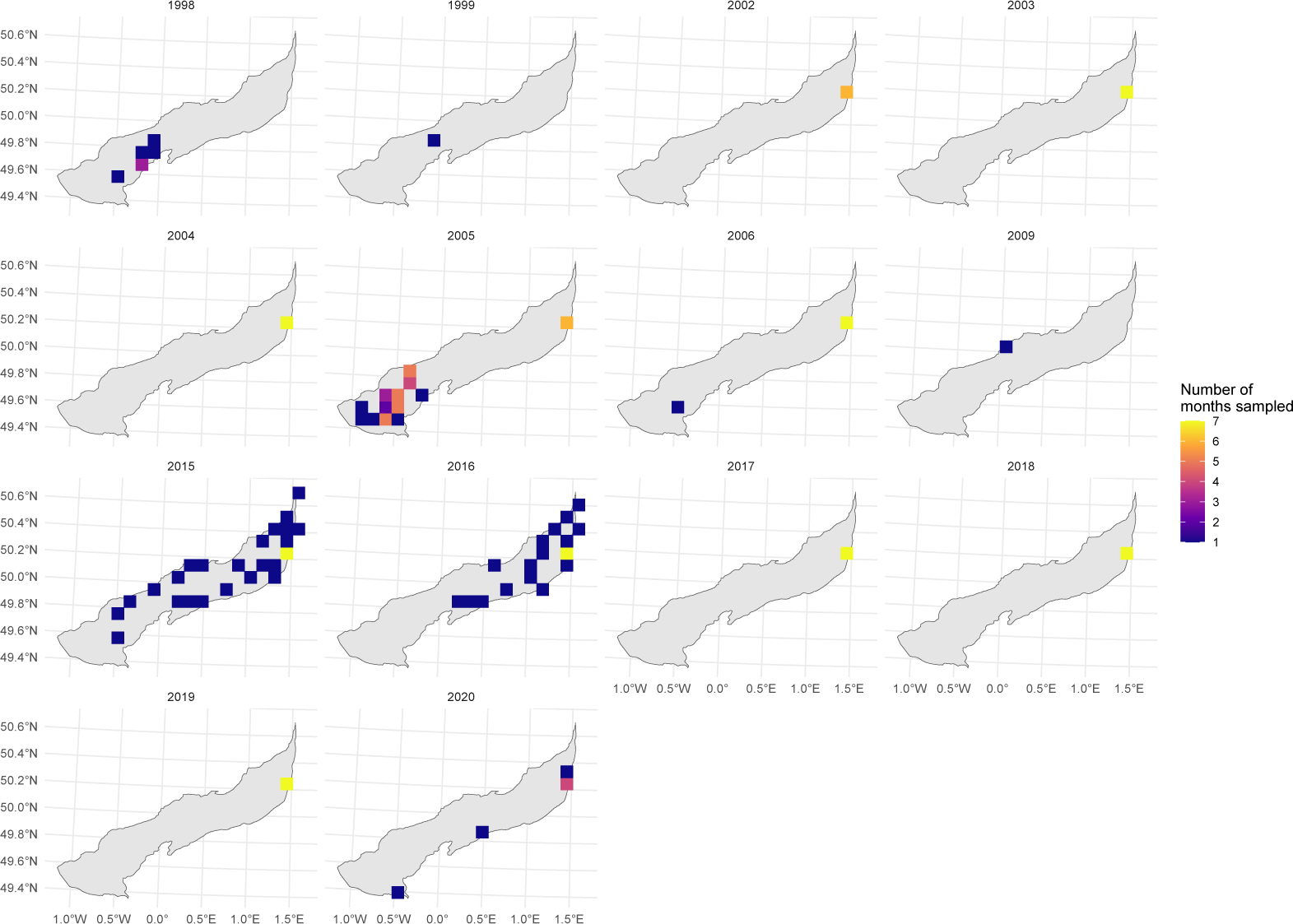
Figure 8. Distribution of in-situ measurements on a 10×10 km grid in the KC assessment area per year from March until September. Colors indicate the number of months a grid cell was sampled during the growing season.
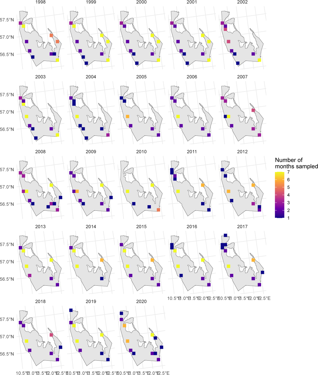
Figure 9. Distribution of in-situ measurements on a 10×10 km grid in the OC assessment area per year from March until September. Colors indicate the number of months a grid cell was sampled during the growing season.
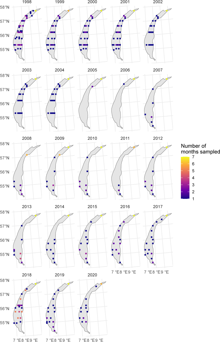
Figure 10. Distribution of EO measurements on a 10×10 km grid in the CFR assessment area per year from March until September. Colors indicate the number of months a grid cell was sampled during the growing season.
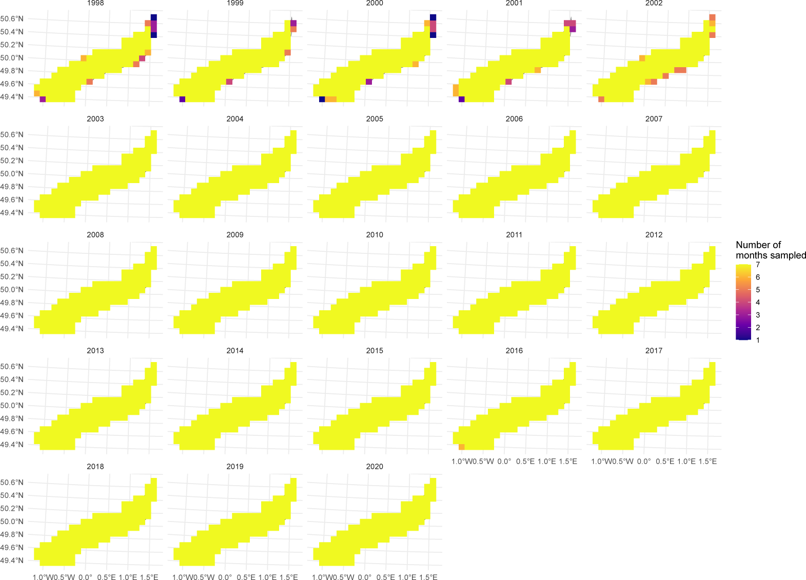
Figure 11. Distribution of EO measurements on a 10×10 km grid in the KC assessment area per year from March until September. Colors indicate the number of months a grid cell was sampled during the growing season.
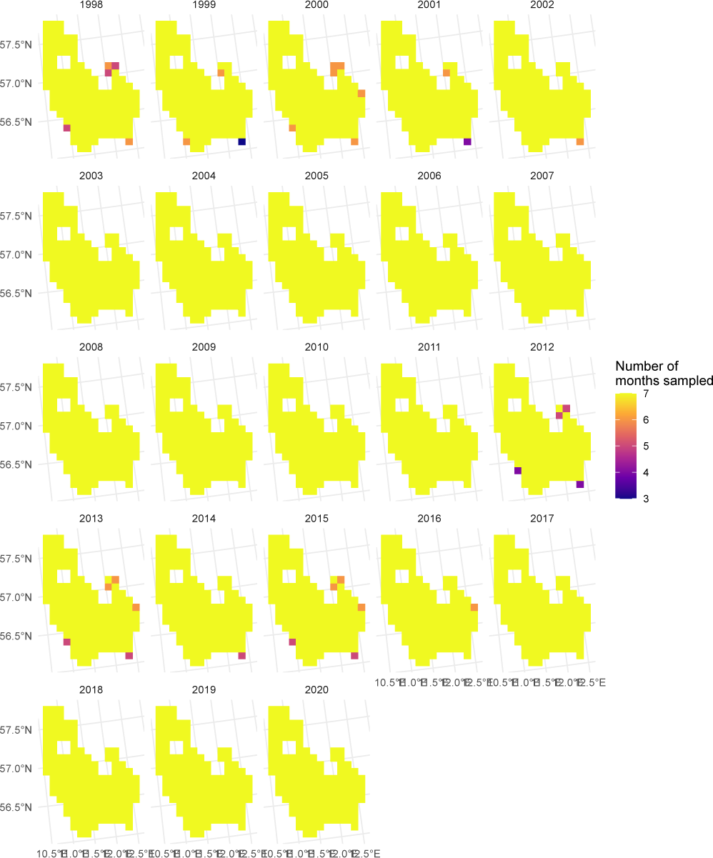
Figure 12. Distribution of EO measurements on a 10×10 km grid in the OC assessment area per year from March until September. Colors indicate the number of months a grid cell was sampled during the growing season.
5.2 Trends
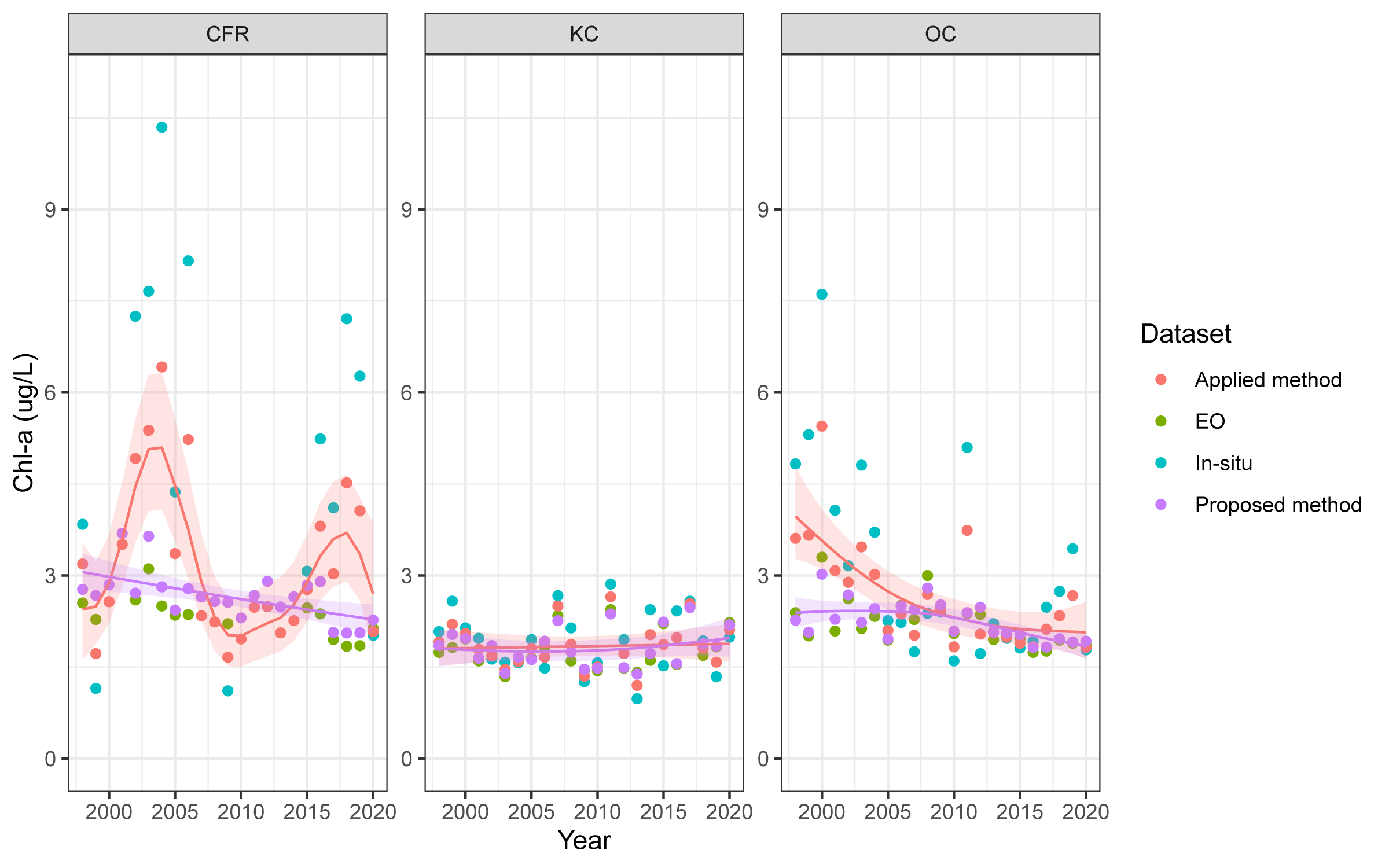
Differences in mean growing season chl-a concentrations between 1998-2020 were assessed for the different methods (Figure 13). The applied approach published on COMPEAT uses a weighted combination of in-situ and EO data (50:50). In contrast, the proposed method first aggregates data on a 10×10 km grid scale per month and year before calculating growing season means. This approach corrects for spatiotemporal sampling biases during the growing season and treats in-situ measurements as individual observations alongside EO data. A 10×10 km grid was chosen in the first aggregation step as the surface area of all three assessments areas was large enough (see section 4).
The two approaches produced differing trends calculated with Trendspotter5) in the CFR and OC.
In the CFR, the 50% weight of in-situ measurements resulted in considerably higher chl-a means in the applied method between 2002–2006 and 2016–2019 compared to the proposed method, with minimal overlap of the 95% confidence intervals over the entire period. In-situ chl-a concentrations during these periods were largely based on only one repeatedly measured sampling site close to the shore. Between 2007 and 2014, almost no in-situ measurements were available, causing the OSPAR chl-a means to exactly follow the EO data. Chl-a means calculated with the proposed method are slightly higher because of the first aggregation step.
In the OC, applying 50% weights to in-situ measurements resulted in higher chl-a means for the applied method between 1998 and 2005 compared to the proposed method, without overlap of the 95% confidence intervals. Although the in-situ sampling points were spatially fairly evenly distributed across the OC during that period, their temporal distribution was not: excluding the repeatedly measured northernmost site, 85% of samples were collected only in April and August, which may have introduced a temporal bias in in-situ chl-a concentrations.
In contrast, in the KC the trends derived from applied method and the proposed method were similar in both EO and in-situ datasets.
Figure 13. Chlorophyll-a growing season means between 1998-2020 for the OSPAR assessment areas CFR, KC and OC. Different colored points show the means according to the in-situ data (blue), EO data (green), and applying the proposed method (purple) or the applied method used by OSPAR (red). For the latter two, trendlines calculated with Trendspotter including a 95% confidence interval are also shown.
5.3 COMP4 assessment
The COMP4 assessment of the chl-a eutrophication status was repeated for the CFR, OC and KC OSPAR assessment areas using the proposed method and compared to the results published on COMPEAT (Table 5). The down-weighting of in-situ data according the confidence rating was not applied on COMPEAT, see annex I for the results in these assessment areas according to the agreed method (on average 70:30 weighting for EO to in-situ data in CFR; although no shifts in status occurred).
To determine the confidence ratings for each area, sample sizes corresponding to error ranges of 10% and 5% were calculated using the relative margin of error (MOE) (see section 4.4 of the previous report6)). For all three areas, the 10% threshold between ‘Low’ and ‘Moderate’ confidence corresponds to a sample size of approximately 50, while the 5% threshold between ‘Moderate’ and ‘High’ confidence corresponds to a sample size of approximately 220.
| Applied method | Proposed method | |||||||||
|---|---|---|---|---|---|---|---|---|---|---|
| Area | Period | TV | Chl-a (ug/L) | EQRS | Status | Confidence rating | Chl-a (ug/L) | EQRS | Status | Confidence rating |
| CFR | 2015-2020 | 2,8 | 3,4 | 0,49 | Moderate | High | 2,0 | 0,91 | High | High |
| KC | 2015-2020 | 1,2 | 2,0 | 0,25 | Poor | High | 2,0 | 0,21 | Poor | High |
| OC | 2015-2020 | 1,6 | 2,1 | 0,39 | Poor | High | 1,9 | 0,46 | Moderate | High |
Figure 14. EQRS for the OSPAR assessment area’s CFR, KC, and OC, between 2015-2020 as applied in COMP4 and according to the proposed method.
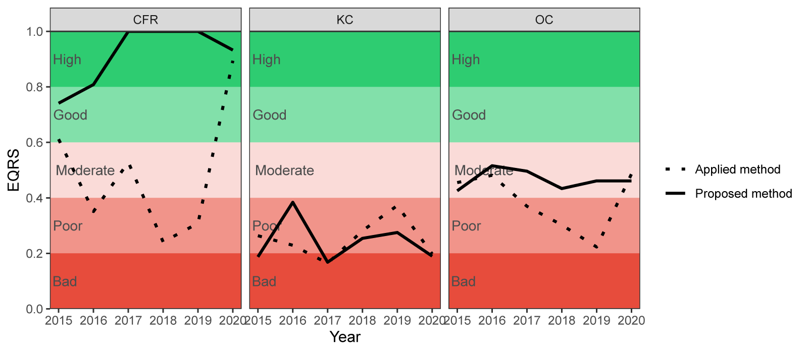
Using our proposed method, mean growing season chl-a concentrations were lower than those reported currently on COMPEAT for the CFR and OC (Table 5). This difference results from the reduced influence of in-situ data, which was more affected by extreme chl-a values due to its smaller sample size and sporadic sampling in these areas compared to the EO data (Figure 13). The reduced weighting of in-situ data leads to higher EQRS values and consequently a more positive eutrophication status: in the CFR, the status improved from Moderate to High, and in the OC from Poor to Moderate. Annual EQRS differences for COMP4 are shown in Figure 14, where EQRS values are generally higher under the proposed method, with status changes observed in several years for the CFR and OC assessment areas.
In contrast, in the KC assessment area, differences between mean chl-a concentrations from EO and in-situ data were less pronounced, resulting in comparable mean growing season values and identical eutrophication status as currently reported on COMPEAT and using the proposed method.
Confidence ratings were high in all three assessment areas using both the applied method and the proposed method.
5.4 Conclusion
The proposed method for assessing mean growing season chl-a concentrations and eutrophication status provides a more spatially and temporally balanced representation of conditions in the CFR, KC, and OC OSPAR assessment areas. By aggregating both in-situ and EO data on a 10×10 km grid scale per month and year, the novel approach corrects for biases caused by uneven sampling frequency and limited spatial coverage, particularly from the in-situ dataset.
In-situ data contributed only a very small fraction of the total measurements and were often concentrated in a few coastal grids, with several years lacking in-situ observations altogether. Consequently, the strong influence of extreme chl-a values in the applied 50:50 weighted approach led to higher mean chl-a concentrations in the CFR and OC compared to the proposed method. By reducing this disproportionate influence, the proposed method produced higher EQRS values and thus a more positive eutrophication status: the CFR improved from a Moderate to a High status, and the OC from a Poor to a Moderate status. In the KC, where in-situ and EO data were more consistent, results between the two approaches were largely comparable.
The application of objective confidence thresholds based on sample size further strengthens the transparency and reproducibility of the evaluation. Boundaries between confidence classes can be set based on the acceptable error range (here 10% and 5%).
Overall, the proposed method enhances the robustness of chl-a eutrophication assessments by providing a more objective and spatiotemporal representative integration of EO and in-situ observations. This approach can serve as a consistent and adaptable framework for future OSPAR assessments, improving comparability across regions and years.
6. Concluding remarks
The present study expands on the proposed methodology developed in the previous CBS report for assessing chl-a and eutrophication status within the OSPAR framework. By first aggregating in-situ and EO data on a year-month-grid basis and deriving confidence ratings from concomitant sample sizes, the method provides a more objective and spatiotemporal representative approach to eutrophication assessment.
Across assessment areas, results consistently showed that mean growing season chl-a concentrations derived with the proposed method were slightly lower and less variable than those currently published on COMPEAT with equal weighting of EO and in-situ data. This reduction reflects the mitigation of biases caused by uneven or limited in-situ sampling, particularly in coastal waters where a few high-value observations can disproportionately influence the mean. Consequently, the proposed method often produced higher EQRS values and, in several cases, a more favorable eutrophication status, while simultaneously providing a clearer indication of the underlying uncertainty through the confidence rating.
The proposed method aligns closely with the direction outlined in OSPAR’s Annex 14: Improving and harmonizing methods for data aggregation in space, time and between data types7), which emphasizes the need for transparent, harmonized procedures to integrate diverse data types and avoid spatial or temporal bias. Similar to examples one and three described there, the method first aggregates EO and in-situ data on a common spatial grid and at a monthly temporal scale before deriving growing-season means. This first aggregation step prevents bias toward high-frequency EO data and ensures that each grid cell and period is represented by a single, balanced statistic with an associated confidence rating. In doing so, it operationalizes the principles OSPAR identified as essential for future eutrophication assessments, combining methodological consistency and transparency, while demonstrating their feasibility in practice. However, unlike the examples in Annex 14, we did not apply separate weighting to combine the different datatypes, because the pronounced spatiotemporal imbalances between EO and in-situ data would have introduced bias.
Analyses of grid resolution further showed that assessment outcomes were largely stable across scales, although spatial detail does decrease at coarser resolutions, particularly in small river plume areas such as MPM and SCHPM2. Using a 5×5 km grid in the first aggregation step might strike a practical balance in these smaller areas: it captures enough spatial representativeness while maintaining sufficient statistical confidence. Based on the results, we recommend that a 5×5 km grid should be applied to areas smaller than 205 km2, and that a 10×10 km grid can be applied to areas larger than 580 km2. Further analysis is needed to determine the exact surface area threshold between resolutions. These insights support a flexible, area-specific approach rather than a one-size-fits-all resolution.
Applying the proposed method beyond the OSPAR areas that overlap with Dutch waters, including CFR, KC, and OC, demonstrated its broader applicability. In these regions, the method again produced more stable and representative chl-a means and eutrophication classifications, reducing the disproportionate influence of limited in-situ measurements.
Overall, the proposed method strengthens the scientific basis of eutrophication assessments under OSPAR by (1) integrating EO and in-situ data in a statistically consistent, spatiotemporally explicit framework, (2) quantifying uncertainty through objective confidence ratings, and (3) providing a transparent and adaptable approach for regions of varying size and data availability. Its implementation would contribute to more consistent and policy-relevant eutrophication assessments across the OSPAR maritime area. In this context, it is important that the right management signals are sent, and therefore the relation of the assessment results to a verified and, if necessary, adjusted eutrophication threshold value must also be correctly established.
Annex I
| Agreed method | Proposed method | |||||||||
|---|---|---|---|---|---|---|---|---|---|---|
| Area | Period | TV | Chl-a (ug/L) | EQRS | Status | Confidence rating* | Chl-a (ug/L) | EQRS | Status | Confidence rating |
| MPM | 2015-2020 | 8 | 11,1 | 0,34 | Poor | Moderate | 9,7 | 0,43 | Moderate | Moderate |
| RHPM | 2015-2020 | 6,8 | 7,6 | 0,53 | Moderate | High | 7,3 | 0,53 | Moderate | Moderate |
| SNS | 2015-2020 | 3,8 | 3,3 | 0,74 | Good | High | 3,0 | 0,83 | High | High |
| SCHPM2 | 2015-2020 | 8,9 | 11,0 | 0,43 | Moderate | Moderate | 11,1 | 0,41 | Moderate | Moderate |
| SCHPM1 | 2015-2020 | 5 | 12,2 | 0,14 | Bad | Moderate | 12,1 | 0,14 | Bad | Moderate |
| CFR | 2015-2020 | 2,8 | 3,0 | 0,54 | Moderate | Moderate | 2,0 | 0,91 | High | High |
| KC | 2015-2020 | 1,2 | 2,0 | 0,25 | Poor | High | 2,0 | 0,21 | Poor | High |
| OC | 2015-2020 | 1,6 | 2,1 | 0,38 | Poor | High | 1,9 | 0,46 | Moderate | High |
| *Average in-situ confidence rating over the period 2015-2020, which determines the weighting when combining in-situ and EO data | ||||||||||