2. Revision figures
2.1 Temporal coverage of in-situ measurements
The previous report illustrated the temporal coverage of in-situ measurements in the SNS assessment area by showing how many months each site was sampled each year, based on the exact coordinates of individual monitoring locations (Figure 1). The challenge with this visualization approach is that the temporal coverage might not align well with the sampling strategy used by some countries, most notably the United Kingdom, which follows a random sampling design rather than fixed monitoring stations. In such cases, multiple measurements may be taken within the same grid cell during a single growing season, even though no fixed location is sampled consistently over time.
To more accurately reflect the temporal coverage of in-situ sampling under such designs, Figure 1 should be revised to show the number of months sampled per grid cell per year, rather than per fixed site. This would better capture the actual sampling effort, particularly in areas where fixed locations are not used (Figure 2). This also aligns better with our improved method, in which growing season means are first aggregated on a grid basis.
Figure 1. Distribution of in-situ measurements in the SNS assessment area per year from March until September. Colors indicate the number of months a site was sampled during the growing season.
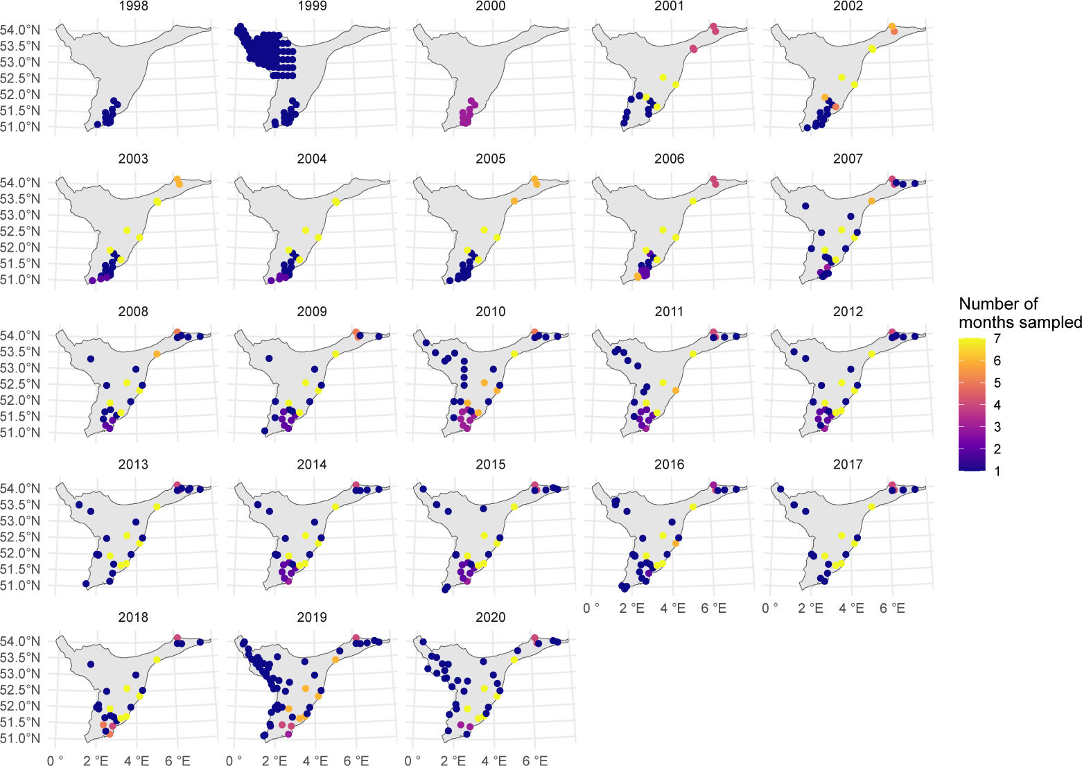
Figure 2. Revision of figure 1 from the previous report, showing the distribution of in-situ measurements on a 25×25 km grid in the SNS assessment area per year from March until September. Colors indicate the number of months a grid cell was sampled during the growing season.
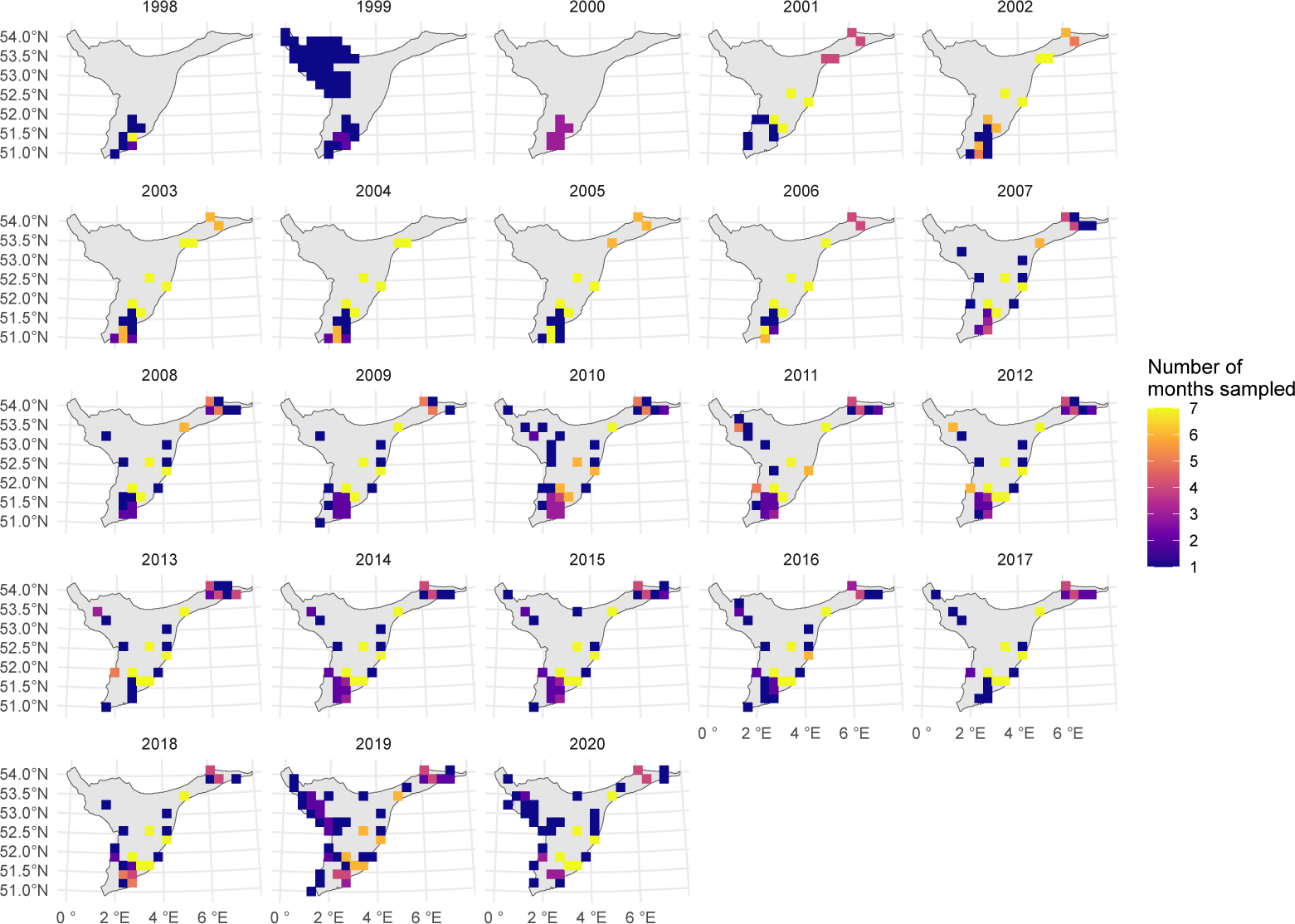
Figure 1 and 2 show that the temporal coverage of in-situ measurements does not differ substantially when comparing grid cell-based data to exact location data. In Figure 1, 784 points are shown using exact coordinates, compared to 518 points using the 25×25 km grid approach (Figure 2). The number of points with repeated measurements is slightly higher in the grid-based version (269) than in the exact location version (252). Similarly, the average number of months sampled per point is marginally higher when using grid cells, with 3 months compared to 2.3 months for exact locations. However, only over half of all the grid cells at a 25×25 km resolution are sampled, when considering just in-situ data. In years when more locations were sampled off the British coast, most measurements were concentrated in one (July 1999) or two months (July/August 2019 and July/September 2020) within the growing season, rather than being distributed across multiple months. Consequently, only minor differences in temporal coverage are expected between the two figures.
2.2 Conclusion
Although the UK employs a random sampling design, measurements do not always occur in different months each year. As a result, a different visualization approach does not greatly improve the overall temporal coverage of in-situ data.
2.3 Trends RHPM and MPM
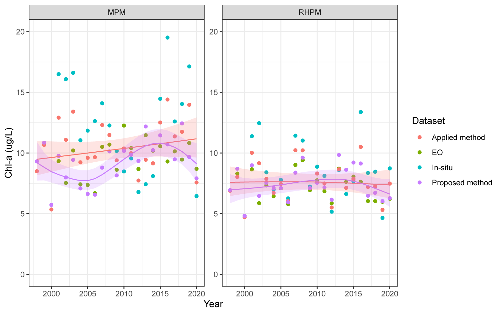
Trends in mean growing season chl-a concentrations between 1998-2020 were assessed for the applied method and the proposed method, but only for the SNS OSPAR assessment area in the previous report (see section 4.3)1). Figure 3 presents these trends, calculated with Trendspotter2), also for the MPM and RHPM areas. Trendspotter is a method to estimate flexible trendlines for time series data. The applied approach uses a weighted combination of in-situ and EO data (50:50). In contrast, the proposed method first aggregates data on a 10×10 km grid scale per month and year before calculating growing season means. This approach corrects for spatiotemporal sampling biases during the growing season and treats in-situ measurements as individual observations alongside EO data.
In the MPM, both methods reveal distinct trends (although with substantial overlap of 95% confidence intervals): while the applied method indicates a steady increase, the proposed method shows a peak around 2015 followed by a decline in recent years. Over time, in-situ chl-a concentrations ranged from 6.8 until 19.5 µg/L, while EO chl-a concentrations ranged from 6.7 until 12.3 µg/L. In-situ data in this assessment area is also only based on one sampling site that is sampled each month during the growing season.
In the RHPM, the trends are more similar, though the post-2015 decrease is more pronounced in the proposed method. Over time, in-situ chl-a concentrations ranged from 4.7 until 13.4 µg/L, while EO chl-a concentrations ranged from 4.7 until 9.4 µg/L. In-situ data in the RHPM is based on three sampling site that are sampled each month during the growing season.
Figure 3. Chlorophyll-a growing season means between 1998-2020 for the OSPAR assessment areas MPM and RHPM. Different colored points show the means according to the in-situ data (blue), EO data (green), and applying the proposed method (purple) or the method applied by OSPAR (red). For the latter two, trendlines calculated with Trendspotter including a 95% confidence interval are also shown.
2.4 Conclusion
Subtle differences are observed in the temporal patterns between the proposed grid-based method and the applied approach used by OSPAR for calculating growing season mean chl-a in the MPM and RHPM assessment areas, although these differences are less pronounced than those found in the previous report for the SNS assessment area.