HSMR 2022 Methodological Report
About this publication
Statistics Netherlands has calculated The Hospital Standardised Mortality Ratios (HSMRs) for Dutch hospitals for the period 2020-2022. This report describes the methods that were used.
The following files are made available in the Appendix: the Excel file ‘Statistical significance of covariates HSMR 2022 model’ presents the statistical significance (95% confidence) of the covariates for the 158 logistic regressions; the Excel file ‘Classification of variables HSMR 2022’ contains the classifications used for the diagnosis groups, severity of main diagnosis, socio-economic status and source of admission and; the Excel file ‘Coefficients HSMR 2022’ contains the coefficients and standard errors of the HSMR model by diagnosis group.
In chapter 2 the changes compared to previous HSMR calculations are described. The largest change in the present HSMR model is that for reporting year 2022 the admissions with COVID-19 as main diagnosis have been included. COVID-19 admissions of 2020 and 2021 are excluded from the HSMR 2020-2022, like in previous HSMR calculations. In chapter 4 the quality of the present HSMR model is evaluated and the effect of including COVID-19 admissions on the HSMRs 2022 is described.
HSMR 2022 outcomes are published by the hospitals (31 December 2023 at the latest), on the websites of the individual hospitals.
1. Introduction
This report presents the methods Statistics Netherlands (CBS) has used to calculate the Hospital Standardised Mortality Ratios (HSMRs) for Dutch hospitals. HSMRs are ratios of observed and expected numbers of deaths and aim to present in-hospital mortality figures in comparison to the national average. This chapter gives a general overview of the HSMR. Chapter 2 presents the changes introduced in the method of calculating the HSMR. The methodological aspects of the model used to calculate the HSMRs are described in chapter 3. The model outcomes are evaluated in chapter 4 and include the evaluation of the model for COVID-19 admissions which was integrated in the HSMR 2022. Conclusions are given in chapter 5.
1.1 What is the (H)SMR?
In-hospital mortality can be measured as the ratio of the number of hospital deaths to the number of hospital admissions (hospital stays) in the same period. This is generally referred to as the “gross mortality rate”. Judging hospital performance on the basis of gross mortality rates is unfair, since one hospital may have had more life-threatening cases than another. Therefore it is more appropriate to adjust (i.e. standardise) mortality rates for differences in patient characteristics (”case mix”) across hospitals as much as possible. To this end, the SMR (Standardised Mortality Ratio) of a hospital h for diagnosis d is defined as
\begin{equation}
\mathrm{SMR}_{dh} = 100 \times \frac{
\textrm{Observed mortality}_{dh}
}{
\textrm{Expected mortality}_{dh}
}
\end{equation}
The numerator is the observed number of deaths with main diagnosis d in hospital h. The denominator is the expected number of deaths for this type of admission under the assumption that individual mortality probabilities (per admission) do not depend on the hospital, i.e. are equal to mortality probabilities of identical cases in other hospitals. The denominator is determined using a model based on data from all national hospitals, in which the in-hospital mortality is explained by patient characteristics, such as age and diagnosis, and characteristics of the admission, such as whether the admission is acute or not. Characteristics of the hospital, such as the number of doctors per bed, are generally not incorporated in the model, since these can be related to the quality of care which is the intended outcome of the indicator. The model thus produces an expected (estimated) mortality probability for each admission. Adding up these probabilities per hospital gives the total expected mortality over all admissions of that hospital. For each diagnosis d, the average SMRd across all hospitals equals 100 when each hospital is weighted with its (relative) expected mortality.
The HSMR of hospital h is defined as
\begin{equation}
\mathrm{HSMR}_{h} = 100 \times \frac{
\textrm{Observed mortality in } h
}{
\textrm{Expected mortality in } h
}
\end{equation}
in which both the numerator and denominator are sums across all admissions for all considered diagnoses. The HSMR thus also has a weighted average of 100. As HSMRs may also deviate from 100 by chance only, confidence intervals are calculated for the SMRs and HSMRs to inform hospitals whether they have a (statistically) significantly high or low adjusted mortality rate compared with the average value of 100.
1.2 Purpose of the HSMR
As in many other countries, there is much interest in measuring the quality of health care in the Netherlands. Various quality indicators are available, such as the number of medical staff per bed or the availability of certain facilities. However, these indicators do not measure the outcomes of medical performance. A good indicator for the performance of a hospital is the extent to which its patients recover, given the diagnoses and other important patient characteristics, such as age, sex and comorbidity. Unfortunately, recovery is hard to measure and mostly occurs after patients have been discharged from the hospital. Although in-hospital mortality is a much more limited quality indicator, it can be measured accurately and is therefore used as a quality indicator in several countries, using the HSMR and SMRs as defined in section 1.1. If these instruments were totally valid, i.e. the calculations would adjust perfectly for everything that cannot be influenced by the hospital, a value above 100 would always indicate inferior quality of care, and the difference between numerator and denominator could be considered an estimate of “avoidable mortality”. This would only be possible if the measurement was perfect and mortality by unforeseeable complications was equally distributed across hospitals, after adjustment for differences in case mix. However, it is impossible to construct such a perfect instrument to measure the quality of health care; the outcome of the indicator will to some extent always be partially influenced by differences between hospitals with regard to case mix, availability of highly specialized treatment options, etc. A significantly high (H)SMR will at most be an indication of possible shortcomings in hospital care, but a high value may also be caused by coding errors in the data or a lack of essential covariates related to mortality in the model. Still, a significantly high (H)SMR is often seen as a warning sign and a reason for further investigation by the hospital.
1.3 History of the HSMR
In 1999 Jarman initiated the calculation of the (H)SMR for hospitals in England (Jarman et al., 1999). In the following years the model for estimating mortality probabilities was improved by incorporating additional covariates. Analogous models were adopted by some other countries.
In 2005, Jarman started to calculate the (H)SMR for the Netherlands. Later on, these Dutch (H)SMRs were calculated by Kiwa Prismant, in collaboration with Jarman and his colleagues of Imperial College London, Dr Foster Intelligence in London and De Praktijk Index in the Netherlands. Their method, described in Jarman et al. (2010), was slightly adapted by Prismant (Prismant, 2008) up to reporting year 2009. In 2010 DHD (Dutch Hospital Data, Utrecht), the registry holder of the national hospital discharge data, asked CBS to calculate the (H)SMRs for the period 2008-2010 and for subsequent years. CBS is an independent public body and is familiar with the input data for the HSMR, i.e. the hospital discharge register (LBZ: Landelijke Basisregistratie Ziekenhuiszorg and its predecessor LMR: Landelijke Medische Registratie), as it uses this data source for a number of health statistics (see https://opendata.cbs.nl/statline/#/CBS/nl/).
The starting point for CBS was the HSMR method previously used by Prismant. As a result of progressive insight, over the years CBS has introduced changes in the model for the HSMR, which are described in the annual methodological reports (CBS, 2011, 2012, 2013, etc.).
1.4 Confidentiality
Under the Statistics Netherlands Act, CBS is required to keep all data about individuals, households, companies or institutions confidential. Therefore it normally does not deliver recognisable data from institutions to third parties, unless the institutions concerned explicitly agree. For this reason, CBS needs written consent from all hospitals to deliver their hospital-specific (H)SMR figures to DHD. CBS only supplies DHD with (H)SMR outcomes of hospitals that have granted authorisation to do so. In turn, DHD sends each hospital its individual outcome report. Publication of (H)SMR data, which has become mandatory in the Netherlands since 2014 by a regulation of the Dutch Healthcare Authority (NZa), is the responsibility of the hospitals themselves. CBS does not publish data on identifiable hospitals.
1.5 CBS output
CBS annually estimates the models for expected mortality per diagnosis for the most recent three-year period. It calculates the HSMRs and SMRs for all hospitals that (1) had authorised CBS, (2) had registered all of its admissions in the LBZ in the relevant period, and (3) were not excluded on the grounds of criteria for data quality and comparability, which means that the hospital’s LBZ data were not too deviant in some respects (see section 3.5).
CBS produces the following output:
- Individual hospital reports, containing their HSMR and diagnosis-specific SMR figures for the most recent reporting year and the three-year period. SMRs are also presented for different patient groups (by age, sex and urgency of admission) and for clusters of diagnoses. Hospitals can compare their outcome with the national average: overall, and per diagnosis and patient group.
- A dataset for each hospital with the mortality probabilities for all its individual admissions. Besides the mortality probability, each admission record contains the observed mortality (0 or 1) and the scores on the covariates of the HSMR model. Hospitals can use these data for internal investigation.
- A report on the methods used for calculating the HSMR, including the model results and parameters (this document; see www.cbs.nl).
1.6 Limitations of the HSMR
In section 1.2 we argued that the HSMR is not the only indicator to measure quality of hospital care. Furthermore, the quality and limitations of the HSMR (and the SMR) instrument are under debate. After all it is based on a statistical model (i.e. the denominator), which is always a simplification of reality.
Since the very first publication on the HSMR in the United Kingdom, there has been an on-going debate about the value of the HSMR as an instrument. Supporters and opponents agree that the HSMR is not a unique, ideal measure, but at most a possible indicator of the quality of health care, alongside other possible indicators. But even if HSMRs were to be used for a more limited purpose, i.e. standardising in-hospital mortality rates for unwanted side-effects, the interpretation of HSMRs would present various problems, some of which are described briefly below. See also Van Gestel et al. (2012) for an overview.
- Section 3.4 contains the list of covariates included in the regression model. Hospitals do not always code these variables in the same way. Variables such as age and sex are registered uniformly, but the registration of whether an admission was acute or not, the main discharge diagnosis or comorbidity may depend on individual physicians and coders. Lilford and Pronovost (2010) argue that if the quality of the source data is insufficient, the regression model should not adjust for such erroneously coded covariates. Our own research (Van der Laan, 2013) shows that comorbidities in particular present a problem in the Netherlands, as there is large variation in coding of this covariate (see also section 4.3). Van den Bosch et al. (2010) refer extensively to the influence of coding errors and Van Erven et al. (2018) also describe underreporting of comorbidities. Nationwide, the registration of comorbidities in Dutch hospitals has increased strongly up to 2014. From 2015 onwards the yearly increase is smaller, and in 2021 the registration of comorbidities seemed to stabilize. However, there are still hospitals with annual shifts in the registration of comorbidities. Exclusion criteria for outliers may solve this problem partly but not completely.
- Another problem is that some hospitals do not sufficiently register whether a comorbidity was a complication or not. As complications are excluded from the HSMR comorbidity covariates, underreporting complications might falsely lead to a higher comorbidity rate, thus influencing the HSMR outcomes. To stimulate correct coding of complications, an indicator has been added to the hospital HSMR reports showing the percentage of registered complications of the hospital, and the overall average. The introduction of this indicator has led to less underreporting of complications, though there are still differences in the number of complications registered by hospitals.
- Some hospitals may, on average, treat more seriously ill patients than others, even if those patients have the same set of scores on the covariates. University hospitals may, for example, have more complicated cases than other hospitals, while regional hospitals are generally more involved in end of life care. It is questionable whether the model sufficiently adjusts for factors such as severity and complexity of disease. As some of the desired covariates, such as disease stage, are not registered in the LBZ and may actually be hard to measure at all in this type of registry with routinely collected hospital discharge data, essential information to correct for differences in case mix between hospitals may be missing.
- A similar problem occurs when certain high-risk surgical procedures are only performed in a selection of hospitals. For instance, open heart surgery only occurs in authorised cardiac centres, and these hospitals may have higher SMRs for heart disease because they perform such risky interventions. This could be solved by including a covariate in the model that indicates whether such a procedure was performed. The downside however, of using a treatment method as a covariate, is that ideally it should not be part of the model as it is a component of hospital care.
- Hospital admission and discharge policies may differ between hospitals. For instance, one hospital may admit the same patient more frequently but for shorter stays than another. Or it may discharge a patient earlier due to higher availability of external terminal care facilities in the neighbourhood. Also, patients may be referred from one hospital to another for further treatment. Obviously, all these situations that mostly are unrelated to quality of care influence the observed mortality numbers and thereby the outcome of the HSMR.
- Hospitals can compare their HSMR and SMRs with the national average value of 100. A comparison of (H)SMRs between two (or more) hospitals is more complicated, as there is no complete adjustment for differences in case mix between pairs of hospitals. Theoretically, it is even possible that hospital A has higher SMRs than hospital B for all diagnosis groups, but a lower HSMR. Although this is rather theoretical, bilateral comparison of HSMRs should be undertaken with caution (Heijink et al., 2008).
Some issues in the incomplete correction for differences in case mix between hospitals may be partly addressed by peer group comparison of (H)SMRs. The calculation of (H)SMRs is still based on the model for all hospitals (without correcting for the type of hospital), but peer group comparison allows a specialised hospital to compare its results with the average for similar hospitals. For instance, the average HSMR of university hospitals is >100 in the Netherlands due to insufficient case mix correction, but comparing their results with a peer group average allows these hospitals (and for specific diagnoses also other specialised hospitals) to better interpret their own scores.
To tackle the problem relating to differences in discharge policies (e.g. the availability of terminal care outside hospital), and to some extent referrals between hospitals, an indicator of early post-discharge mortality could be included, in addition to in-hospital mortality. Ploemacher et al. (2013) observed a decrease in standardised in-hospital mortality in the Netherlands in 2005-2010, which may have been caused by an overall improvement in quality of care, but may also be partly explained by substitution of in-hospital mortality by outside-hospital mortality, possibly caused by changes in hospital admission and discharge policies. Pouw et al. (2013) performed a retrospective analysis on Dutch hospital data linked to mortality data, and concluded that including early post-discharge mortality diminishes the effect of discharge bias on the HSMR. In the UK, the SHMI (Summary Hospital-level Mortality Indicator) has been adopted, which includes mortality up to 30 days after discharge (Campbell et al., 2011). In 2014, CBS studied the optimal time frame and definition of an indicator including early post-discharge mortality (Van der Laan et al., 2015). Including all mortality within a 45-day period after admission was advised to reduce the influence of hospital discharge policies on the HSMR. A French study also recommended fixed post-admission periods of more than 30 days (Lamarche-Vadel et al., 2015).
However, including post-discharge mortality in the indicator will not reduce the effect of differences in admission policies for terminally ill patients. Some hospitals may admit more terminally ill patients to provide terminal palliative care than other hospitals and those admissions may distort HSMR outcomes. Palliative care in general can be measured in ICD-10 (code Z51.5), but this variable should be used with caution, as differences between hospitals in coding practices have been shown in e.g. the UK and Canada, and adjusting the HSMR for palliative care may increase the risk of gaming (NHS, 2013; Chong et al., 2012; Bottle et al., 2011). Because of this, and because ICD-10 code Z51.5 does not distinguish between early and terminal palliative care, palliative care admissions have not yet been excluded from the calculation of the HSMR in the Netherlands. However, the hospital HSMR reports include information on the percentage of the hospital’s admissions and deaths related to palliative care as registered in the LBZ compared to the overall average. This may indicate to some extent whether or not palliative care could have biased a hospital’s HSMR. However, since in the Netherlands there is also a large variation between hospitals in the coding of palliative care, this information should be used with caution. Because of the limitations of using code Z51.5 as an indicator of palliative care, other indicators may be considered for inclusion in future HSMR-models.
Despite the above-mentioned limitations and the ongoing debate on the validity and reliability of mortality-based indicators like the HSMR, there are studies that suggest that mortality monitoring can be indicative of failings in quality of care. In an English hospital setting, Cecil et al. (2020) found that mortality alerts, based on higher than expected mortality in 122 diagnosis and procedure groups, were associated with structural indicators of lower quality of care (e.g. lower nurse-to-bed ratio, overcrowding and financial pressures) and outcome indicators like lower patient and trainee satisfaction. They conclude that a mortality alerting system might be valuable in highlighting poor quality of care.
2. Method changes
This chapter summarizes the changes in the HSMR method (HSMR 2022) compared to the method used last year (HSMR 2021). For previous changes see the respective methodological reports (CBS, 2011, …, 2022). Overall, the method has remained the same. Only a few changes related to selection of the data and related to the covariates have been implemented. These changes are described below.
2.1 Inclusion of COVID-19 admissions of 2022
The COVID-19 pandemic significantly impacted hospital care in 2020 and 2021. Because of the different nature of admissions with COVID-19 as a main diagnosis compared to other admissions and the lack of specific expertise for treating COVID-19 during the first months of the pandemic, the COVID-19 admissions were excluded from the HSMR models of 2020 and 2021. This decision was made in agreement with the Dutch Healthcare Authority (NZa) and the Health and Youth Care Inspectorate (IGJ). In 2022 Statistics Netherlands developed a COVID-19 SMR model using 2021 data, which had good predictive power (CBS, 2022). Because of this, and since hospitals have gained experience in treating COVID-19 patients and COVID-19 admissions have been more integrated in regular hospital care in 2022, the newly developed COVID-19 model has now been integrated in the overall HSMR model. The definitions of the covariates in the COVID-19 model is the same as for the models of the other diagnosis groups, except for the covariates “Severity of the main diagnosis” and “Month of admission” (see section 3.4).
Admissions with a main diagnosis of COVID-19 include those with ICD-10 code U07.1 (COVID-19, virus identified (lab confirmed)), U07.2 (COVID-19, virus not identified (clinically diagnosed)) and U10.9 (Multisystem inflammatory syndrome associated with COVID-19, unspecified). In accordance with the HSMR 2020 and 2021, the COVID-19 admissions of 2020 and 2021 were excluded from the present HSMR model which comprises the years 2019-2022. The COVID-19 admissions of 2020 and 2021 were also excluded from the dataset that was used to evaluate data quality and case mix (see section 3.5). For 2022 the COVID-19 admissions were included in the HSMR model and the additional analyses.
Since COVID-19 admissions were only included for the year 2022 (and not for the years 2020 and 2021), the HSMR value of 2022 might be less comparable to the values of the previous years. In section 4.5 the influence of the inclusion of the COVID-19 admissions on the HSMR outcomes is described.
2.2 Exclusion of admissions of healthy persons
From now on all admissions of so-called ‘healthy persons’ are excluded from the HSMR model (for all model years) and additional analyses.
Admissions of healthy persons are admissions of healthy newborns, healthy parents accompanying sick children, or other healthy boarders. These admissions are identified by the main diagnosis of the admission (ICD-10 code Z76.2-Z76.4) and/or the registration of procedure codes for a stay of a healthy newborn or healthy mother for each individual day of the admission ((Dutch procedure codes 190032, 190033 (‘Zorgactiviteiten’ codes), 339911 or 339912 (‘CBV’ codes)).
Since the admissions of healthy persons are non-medical admissions it is not relevant to include these admissions in the HSMR. These admissions are also excluded from other indicators based on the LBZ, such as the hospital readmission rate.
2.3 Updated socioeconomic status (SES) scores for all model years
In the previous HSMR model of 2021 a new variable was used for the socioeconomic status (SES) covariate (see CBS, 2022). This new variable, based on the so-called ‘SES-WOA’ score calculated by Statistics Netherlands (Arts et al., 2022), was introduced because the old variable of the Netherlands Institute for Social Research (SCP) is not updated anymore by SCP. In the HSMR 2021 model the new variable was only applied to the data of 2021. For the earlier years in the model the SES covariate was still based on the SCP variable. However, due to differences in the calculation of the scores, the SCP and SES-WOA scores are not fully comparable.
Therefore, in the current HSMR 2022 model the new SES-WOA variable was applied to all model years (2019-2022). For the model years 2019-2021 the SES-WOA scores of 2019 were used and for model year 2022 the SES-WOA scores of 2022 were applied. Further details of the SES-WOA variable are described in section 3.4.
3. (H)SMR model
Expected in-hospital mortality - i.e. the denominator of the SMR - has to be determined for each diagnosis group. To this end we use logistic regression models, with mortality as the target (dependent) variable and various variables available in the LBZ as covariates. The regression models to calculate the (H)SMR of a three-year period (year t-2 up to year t), and the (H)SMRs of the individual years t-2, t-1 and t, are based on LBZ data of four years: year t-3 up to year t. The addition of an additional year (t-3) increases the stability and accuracy of the estimates, while the moving four-year period up to year t keeps the model up to date.
3.1 Target population and dataset
3.1.1 Hospitals
“Hospital” is the primary observation unit. Hospitals register data on admissions (hospital stay data) in the LBZ. However, not all hospitals participate in the LBZ. In principle, the HSMR model includes all short-stay hospitals with inpatient admissions participating in the LBZ in the relevant years. The target population of hospitals that qualify for entry in the HSMR model thus includes all general hospitals, all university hospitals, and short-stay specialised hospitals with inpatient admissions that participate in the LBZ. In case of partial non-response by hospitals, only the fully registered months are included in the model, as in the other months fatal cases might be registered completely and non-fatal cases partially. The partially registered months of those hospitals are removed from the model as these might otherwise unjustly influence the estimates. In addition, if for any reason registered data of hospitals in a specific LBZ year had not been not validated by DHD, that year of data is not included in the HSMR model.
All of the above-mentioned hospitals were included in the model. Data of a short-stay specialised hospital that started registering data in the LBZ in 2022 were also included. (H)SMRs were only calculated for hospitals that met the criteria for LBZ participation, data quality and case mix (see section 3.5).
3.1.2 Admissions
In addition to the population of hospitals, the population of admissions is considered. Our target population of admissions consists of all hospital stays (i.e. inpatient admissions, and prolonged observations, unplanned, without overnight stay) of Dutch residents in Dutch hospitals in a certain period, except admissions that do not meet the billing criteria of the Dutch Healthcare Authority for inpatient admissions, prolonged observations, and admissions of healthy persons, such as healthy newborns, healthy parents accompanying sick children, or other healthy boarders. The date of discharge, and not the day of admission, determines the year a record is assigned to. So the population of hospital stays of year t comprises all admissions that ended in year t. For the sake of convenience, mostly we call these hospital stays “admissions”, thus meaning the hospital stay instead of only its beginning. Day admissions are excluded as these are in principle non-life-threatening cases with hardly any mortality. However, from 2015 onwards the new case type “prolonged observations, unplanned, without overnight stay” is included in the HSMR. This case type was introduced by the Dutch Healthcare Authority (NZa), and replaces the majority of the acute one-day inpatient admissions that had formerly been registered. It involves more mortality than day cases, and it is therefore relevant to include this case type in the HSMR.
Admissions that do not meet the billing criteria of the Dutch Healthcare Authority are removed from the data in all consecutive model years. This primarily concerns one-day inpatient admissions where the patient returned home after discharge. Also, about 100 in-hospital deaths where the patient was admitted after 20:00 hrs. and died before 24:00 hrs. on the same day, were removed from the dataset.
Admissions of healthy persons are additionally removed. These admissions are identified by the main diagnosis of the admission (ICD-10 code Z76.2-Z76.4) and/or the registration of procedure codes for a stay of a healthy newborn or healthy mother for each individual day of the admission ((Dutch procedure codes 190032, 190033 (‘Zorgactiviteiten’ codes), 339911 or 339912 (‘CBV’ codes)).
For the years 2020 and 2021 all admissions with COVID-19 as the principal diagnosis (ICD-10 codes U07.1 (COVID-19, virus identified (lab confirmed)), U07.2 (COVID-19, virus not identified (clinically diagnosed)) and U10.9 (Multisystem inflammatory syndrome associated with COVID-19, unspecified)) were removed from the dataset (see section 2.1).
Lastly, admissions of foreigners are excluded from the HSMR model, partly in the context of possible future modifications of the model, when other data can be linked to admissions of Dutch residents. The number of admissions of foreigners is relatively small.
3.2 Target variable (dependent variable)
The target variable for the regression analysis is the “in-hospital mortality”. As this variable is binary, logistic regressions were performed.
3.3 Stratification
Instead of performing one logistic regression for all admissions, we performed a separate logistic regression for each of the diagnosis groups d. These sub-populations of admissions are more homogeneous than the entire population. Hence, this stratification may improve the precision of the estimated mortality probabilities. As a result of the stratification, covariates are allowed to have different regression coefficients across diagnosis groups.
The diagnosis groups are clusters of ICD codes registered in the LBZ. Here the main diagnosis of the admission is used, i.e. the main reason for the hospital stay, which is determined at discharge. The basis for the clustering is the CCS (Clinical Classifications Software1)), which clusters ICD diagnoses into 259 clinically meaningful categories. The COVID-19 admissions were arbitrarily assigned to group number 260, although this group is originally assigned to external causes of disease by the Clinical Classifications Software. But since external causes of disease cannot be registered as main diagnosis (only as secondary diagnosis) in the LBZ this does not cause any conflict in the data. For the HSMR, we further clustered these 260 categories into 158 diagnosis groups (where the new group 158 consists of the COVID-19 admissions), which are partly the same clusters used for the SHMI (Summary Hospital-level Mortality Indicator) in the UK (HSCIC, 2016). Therefore, the model includes 158 separate logistic regressions, one for each diagnosis group d selected.
In the file “Classification of variables”, published together with this report, for each of the 158 diagnosis groups the corresponding CCS group(s) are given, as well as the ICD-10 codes of each CCS group.
Apart from the SMRs for each of the 158 diagnosis groups, hospitals also receive SMRs for 17 aggregates of diagnosis groups. This allows the evaluation of SMR outcomes at both the detailed and the aggregated diagnosis level. The 17 main clusters are also given in the “Classification of variables” file. These were derived from the main clusters in the CCS classification of HCUP, with the following adaptations:
- HCUP main clusters 17 (“Symptoms; signs; and ill-defined conditions and factors influencing health status”) and 18 (“Residual codes; unclassified”) were merged into one cluster.
- CCS group 54 (“Gout and other crystal arthropathies”) is classified in main cluster “Diseases of the musculoskeletal system and connective tissue”, and CCS group 57 (“Immunity disorders”) is classified in main cluster “Diseases of the blood and blood-forming organs”, whereas in the HCUP classification these groups fall in main cluster “Endocrine, nutritional and metabolic diseases, and immunity disorders”.
- CCS group 113 (“Late effects of cerebrovascular disease”) is classified in main cluster “Diseases of the nervous system and sense organs”, whereas in the HCUP classification this group falls in main cluster “Diseases of the circulatory system”.
- CCS group 218 (“Liveborn”) is classified in main cluster “Complications of pregnancy, childbirth, and the puerperium; liveborn”, whereas in the HCUP classification this group falls in main cluster “Certain conditions originating in the perinatal period”.
- COVID-19 (group 158) was added to the main cluster “Infectious and parasitic diseases”.
These adaptations are in accordance with the diagnosis groups used for the SHMI (Summary Hospital-level Mortality Indicator) in the United Kingdom (HSCIC, 2016).
Although the names of the main clusters are quite similar to the names of the chapters of the ICD-10, there is no one-to-one relation between the two. Although most ICD-10 codes of a CCS group do fall within one ICD-10 chapter, often some of the codes are categorised in other chapters. Especially the codes from the R chapter of ICD-10 are scattered over several HCUP main clusters.
3.4 Covariates (explanatory variables or predictors of in-hospital mortality)
By including covariates of patient and admission characteristics in the model, the in-hospital mortality and thus the (H)SMRs are adjusted for these characteristics. Thus, variables (available in the LBZ) associated with patient in-hospital mortality are chosen as covariates. The more the covariates discriminate between hospitals, the larger the effect on the (H)SMR.
The LBZ variables that are included in the model as covariates are age, sex, socioeconomic status, severity of the main diagnosis, urgency of admission, Charlson comorbidities, source of admission, year of discharge and month of admission. These variables are described below. Detailed classifications of the variables socioeconomic status, severity of the main diagnosis and source of admission are provided in the file “Classification of variables”, published together with this report.
For the regressions, all categorical covariates are transformed into dummy variables (indicator variables), having scores of 0 or 1. A patient scores 1 on a dummy variable if he/she belongs to the corresponding category, and 0 otherwise. As the dummy variables for a covariate are linearly dependent, one dummy variable is left out for each categorical covariate. The corresponding category is the so-called reference category. We took the first category of each covariate as the reference category.
The general procedure for collapsing categories is described in section 3.6.2. Special (deviant) cases of collapsing are mentioned below.
Age at admission (in years): 0, 1-4, 5-9, 10-14, …, 90-94, 95+.
Sex of the patient: male, female.
If Sex is unknown, “female” was imputed. This is a rare occurrence.
SES (socioeconomic status) of the postal area of patient’s home address: lowest, below average, average, above average, highest, unknown.
The SES variable was added to the LBZ dataset on the basis of the postal code of the patient’s residence, as registered in the LBZ. The SES classification is derived from the so called ‘SES-WOA’ scores calculated by Statistics Netherlands (Arts et al., 2022). This SES-WOA score is based on household data concerning welfare (a combination of income and wealth), level of education and recent labour participation. The scores are determined at the household level and then averaged to scores per four-digit postal code. Household-weighted quintiles were calculated from these scores, resulting in the six SES categories mentioned above. Patients for whom the postal area does not exist in the dataset (category “unknown”), were added to the category “average” if collapsing was necessary.
For the HSMR model years 2019-2021 the SES-WOA scores of 2019 calculated by Statistics Netherlands were used and for model year 2022 the SES-WOA scores of 2021 were used.
Severity of the main diagnosis groups: [0-0.01), [0.01-0.02), [0.02-0.05), [0.05-0.1), [0.1-0.2), [0.2-0.3), [0.3-0.4), [0.4-1], Other.
COVID-19_subdiagnosis (for diagnosis group 158 (COVID-19), instead of ‘Severity of the main diagnosis’): U07.1, U07.2, U10.9
The ”Severity of the main diagnosis” covariate is a categorisation of main diagnoses into mortality rates. For the diagnosis groups 1-157, each ICD-10 main diagnosis code is classified in one of these groups, as explained below.
Most of the diagnosis groups have many subdiagnoses (individual ICD-10 codes), which may differ in severity (mortality risk). To classify the severity of the subdiagnoses, we used the method suggested by Van den Bosch et al. (2011), who suggested categorising the ICD codes into mortality rate categories. To this end, we computed inpatient mortality rates for all occurring ICD subdiagnoses of the admissions in the current model years, using data of six historical LBZ years, and chose the following boundaries for the mortality rate intervals: 0, .01, .02, .05, .1, .2, .3, .4 and 1. (“0” means 0 percent mortality; “1” means 100 percent mortality). These boundaries are used for all individual ICD codes. The higher severity categories only occur in a few diagnosis groups. Six historical LBZ years are used to determine this classification, not overlapping with the years the HSMR is calculated for as otherwise both are using the same mortality data. The period of the historical dataset shifts every year for each new HSMR calculation, to keep it up to date.
For newly added ICD-10 codes in recent years a converted “old” ICD-10 code (code used for the disease prior to the introduction of the new ICD-10 code) was determined, in consultation with DHD. If such an ICD-10 code did not occur in the historical dataset, a severity of ”other” was assigned in the calculation of the (H)SMR. ICD codes that are used by less than four hospitals and/or have less than 20 admissions were also set to ”other”. The category ”other” contains diagnoses for which it is not possible to accurately determine the severity. However, if this category “other” needs to be collapsed (see section 3.6.2), it does not have a natural nearby category. We decided to collapse “other” with the category with the highest frequency (i.e. the mode), if necessary. In the file with regression coefficients (see section 4.5) this will result in a coefficient for “other” equal to that of the category with which “other” is collapsed. The only exceptions are when Comorbidity 17 (Severe liver disease) is collapsed with Comorbidity 9 (Liver disease), and when Comorbidity 11 (Diabetes complications) is collapsed with Comorbidity 10 (Diabetes). In these cases the regression coefficient of Comorbidity 17/11 is set to zero in the coefficients file, and the coefficient of the less severe analogue (Comorbidity 9/11) should be used for Comorbidity 17/11.
The individual ICD-10 codes with the corresponding severity categories are available in the separate file “Classification of variables”, published together with this report.
The COVID-19 diagnosis group (nr. 158) consists of only three ICD-10 codes (U07.1, U07.2, and U10.9) that are valid since 2020. As COVID-19 is a new disease, mortality data of previous years does not exist for these codes. Therefore, the three ICD-10 codes of diagnosis group 158 were as such included as separate categories of the severity covariate “COVID-19_subdiagnosis”. This covariate is used in the model of the COVID-19 diagnosis group only, instead of the covariate ”Severity of the main diagnosis”.
Urgency of the admission: elective, acute.
The definition of an acute admission is: an admission that cannot be postponed, as immediate medical treatment or aid within 24 hours is necessary. Within 24 hours means 24 hours from the moment the specialist decides that acute admission is necessary.
Comorbidity 1 – Comorbidity 17. All these 17 covariates are dummy variables, having categories: 0 (no) and 1 (yes).
The 17 comorbidity groups are listed in table 3.4.1, with their corresponding ICD-10 codes. These are the same comorbidity groups as in the Charlson index. However, separate dummy variable are used for each of the 17 comorbidity groups.
All secondary diagnoses registered in the LBZ and belonging to the 17 comorbidity groups are used, but if the ICD-10 code of a secondary diagnosis is identical to that of the main diagnosis, it is not considered a comorbidity. Secondary diagnoses registered as a complication arising during the hospital stay are not counted as a comorbidity either.
In conformity with the collapsing procedure for other covariates (see section 3.6.2), comorbidity groups registered in fewer than 50 admissions or that have no deaths are left out, as the two categories of the dummy variable are then collapsed. An exception was made for Comorbidity 17 (Severe liver disease) and Comorbidity 11 (Diabetes complications). Instead of leaving out these covariates in the case of fewer than 50 admissions or no deaths, they are first added to the less severe analogues Comorbidity 9 (Liver diseases) and Comorbidity 10 (Diabetes), respectively. If the combined comorbidities still have fewer than 50 admissions or no deaths, then these are dropped after all.
The ICD-10 definitions listed in table 3.4.1 are mostly identical or nearly identical to those of Quan et al. (2005), with some adaptations, which are described in CBS (2014). Furthermore, newly introduced ICD-10 codes have been added by CBS if the corresponding ‘old’ ICD-10 code is part of a comorbidity group.
In 2022 two ICD-10 codes (B18.0 and B18.1) were expanded into four 5-digit codes (B18.00, B18.09, B18.10 and B18.19). These subcodes are part of the B18-series, which was already assigned to comorbidity group 9 (liver disease).
| No. | Comorbidity groups | ICD-10 codes |
|---|---|---|
| 1 | Myocardial infarction | I21, I22, I25.2 |
| 2 | Congestive heart failure and cardiomyopathy | I50, I11.0, I13.0, I13.2, I25.5, I42, I43, P29.0 |
| 3 | Peripheral vascular disease | I70, I71, I73.1, I73.8, I73.9, I77.1, I79.0, I79.2, K55.1, K55.8, K55.9, Z95.8, Z95.9, R02, Z99.4 |
| 4 | Cerebrovascular disease | G45.0-G45.2, G45.4, G45.8, G45.9, G46, I60-I69 |
| 5 | Dementia | F00-F03, F05.1, G30, G31.1 |
| 6 | Pulmonary disease | J40-J47, J60-J67 |
| 7 | Connective tissue disorder | M05, M06.0, M06.3, M06.9, M32, M33.2, M34, M35.3 |
| 8 | Peptic ulcer | K25-K28 |
| 9 | Liver disease | B18, K70.0-K70.3, K70.9, K71.3-K71.5, K71.7, K73, K74, K76.0, K76.2-K76.4, K76.8, K76.9, Z94.4 |
| 10 | Diabetes | E10.9, E11.9, E12.9, E13.9, E14.9 |
| 11 | Diabetes complications | E10.0-E10.8, E11.0-E11.8, E12.0-E12.8, E13.0-E13.8, E14.0-E14.8 |
| 12 | Hemiplegia or paraplegia | G04.1, G11.4, G80.1, G80.2, G81, G82, G83.0-G83.5, G83.8, G83.9 |
| 13 | Renal disease | I12.0, I13.1, N01, N03, N05.2-N05.7, N18, N19, N25, Z49.0-Z49.2, Z94.0, Z99.2 |
| 14 | Cancer | C00-C26, C30-C34, C37-C41, C43, C45-C58, C60-C76, C81-C85, C86.0-C86.6, C88, C90-C97, D47.5 |
| 15 | HIV | B20-B24, O98.7 |
| 16 | Metastatic cancer | C77-C80 |
| 17 | Severe liver disease | I85.0, I85.9, I86.4, I98.2, I98.3, K70.4, K71.1, K72.1, K72.9, K76.5, K76.6, K76.7 |
Source of admission: home, nursing home or other institution, (other) hospital.
This variable indicates the patient’s location before admission.
Year of discharge: 2019, 2020, 2021, 2022.
Inclusion of the year of discharge guarantees that the total number of observed and expected (predicted) deaths are equal for that year. As a result the yearly (H)SMRs have an average of 100 when weighting the hospitals proportional to their expected mortality.
As the COVID-19 admissions were included for 2022 only, the covariate “Year of discharge” was not included in the HSMR 2022 model of the COVID-19 diagnosis group (nr. 158).
Month of admission:
- For diagnosis groups 1-157 there are 6 categories:
January/February, …,November/December. - For diagnosis group 158 (COVID-19) there are 13 categories:
0-before 2022, 1-January, 2-February, …, 12-December.
For diagnosis groups 1-157 the months of admission are combined into 2-month periods. For the COVID-19 diagnosis group (nr. 158), however, a more detailed variant of month of admission is used, consisting of 13 values: one for each individual month and a separate category ‘before 2022’ for admissions that started in the year prior to 2022 (and ended in 2022). This more detailed variable allows the COVID-19 model to more distinctly adjust for the effects of different transmission waves. The category for admissions that started in the year prior to 2022 (e.g. in December of 2021) allows the model to distinguish those admissions from admissions that started in the same month in 2022.
3.5 Exclusion criteria
Although all hospitals mentioned in section 3.1.1 are included in the model, HSMR outcome data were not produced for all hospitals. HSMRs were only calculated for hospitals that met the criteria for LBZ participation, data quality and case mix. In addition to this, only HSMRs were calculated for hospitals that had authorised CBS to supply their HSMR figures to DHD.
The criteria for excluding a hospital from calculating HSMRs, based on the characteristics of the registered inpatient admissions and prolonged observations without overnight stay, were:
Insufficient participation in the LBZ
- Hospitals are excluded if they do not register all inpatient admissions and “prolonged observations, unplanned, without overnight stay” that meet the billing criteria of the Dutch Healthcare Authority (NZa) in the LBZ.
Data quality
Hospitals are excluded if:
- ≤30% of admissions are coded as acute.
- ≤1.5 secondary diagnoses are registered per admission, on average per hospital.2)
Case mix
Hospitals are excluded if:
- Observed mortality is less than 60 in all registered admissions.
For 2020 and 2021, admissions with COVID-19 as main diagnosis were excluded from the dataset that was used to calculate the outcomes of the data quality and case mix criteria. For 2022 the COVID-19 admissions were included in this dataset.
In addition to the above-mentioned criteria, hospitals are also excluded if they had not authorised CBS to supply their HSMR figures.
3.6 Computation of the model and the (H)SMR
3.6.1 SMR and HSMR
According to the first formula in section 1.1, the SMR of hospital h for diagnosis d is written as
\begin{equation}
\mathrm{SMR}_{dh} = 100 \frac{O_{dh}}{E_{dh}}
\end{equation}
with Odh the observed number of deaths with diagnosis d in hospital h, and Edh the expected number of deaths in a certain period. We can denote these respectively as
\begin{equation}
O_{dh} = \sum_i D_{dhi}
\end{equation}
and
\begin{equation}
E_{dh} = \sum_i \hat{p}_{dhi}
\end{equation}
where Ddhi denotes the observed mortality for the ith admission of the combination (d,h), with scores 1 (death) and 0 (survival), and p̂dhi the mortality probability for this admission, as estimated by the logistic regression of “mortality diagnosis d” on the set of covariates mentioned in section 3.4 This gives
\begin{equation}
\hat{p}_{dhi} = \mathrm{Prob}\left(D_{dhi} = 1 | X_{dhi} \right) =
\frac{1}{1 + \exp(-\hat{\beta}'_d X_{dhi})}
\end{equation}
with Xdhi the scores of admission i of hospital h on the set of covariates, and the maximum likelihood estimates of 𝛽d, the corresponding regression coefficients, i.e. the so-called log-odds.
For the HSMR of hospital h, we have accordingly
\begin{equation}
\mathrm{HSMR}_h = 100\frac{O_h}{E_h} =
100\frac{\sum_d O_{dh}}{\sum_d E_{dh}} =
100\frac{\sum_d\sum_i D_{dhi}}{\sum_d\sum_i \hat{p}_{dhi}}
\end{equation}
It follows from the above formulae that:
\begin{equation}
\mathrm{HSMR}_h = 100 \frac{
\sum_d E_{dh} \frac{O_{dh}}{E_{dh}}
}{
E_h
} =
\sum_d \frac{E_{dh}}{E_h} \mathrm{SMR}_{dh}
\end{equation}
Hence, an HSMR is a weighted mean of the SMRs, with the expected mortalities across diagnoses as the weights.
3.6.2 Modelling and model-diagnostics
We estimated a logistic regression model for each of the 158 CCS diagnosis groups, using the categorical covariates mentioned in section 3.4. Computations were performed using the glm routine of the statistical software R (R Core Team, 2015). Categories, including the reference category, are collapsed if the number of admissions is smaller than 50 or when there are no deaths in the category, to prevent standard errors of the regression coefficients becoming too large. This collapsing is performed starting with the smallest category, which is combined with the smallest nearby category, etc. For variables with only two categories collapsing results in dropping the covariate out of the model (except for comorbidities 17 (Severe liver disease) and 11 (Diabetes complications) which are first combined with comorbidity 9 (Liver disease), and comorbidity 10 (Diabetes), respectively; see section 3.4). Non-significant covariates are preserved in the model, unless the number of admissions is smaller than 50 (or if there are no deaths) for all but one category of a covariate. All regression coefficients are presented in a file published together with this report.
The following statistics are presented to evaluate the models:
- standard errors for all regression coefficients (published with the regression coefficients);
- statistical significance of the covariates with significance level α=.05, i.e. confidence level .95 (see “Statistical significance of covariates HSMR 2022 model” published together with this report);
- Wald statistics for the overall effect and the significance testing of categorical variables;
- C-statistics for the overall fit. The C-statistic is a measure for the predictive validity of, in our case, a logistic regression. Its maximum value of 1 indicates perfect discriminating power and 0.5 discriminating power not better than expected by chance, which will be the case if no appropriate covariates are found. We present the C-statistics as an evaluation criterion for the logistic regressions.
In addition to these diagnostic measures for the regressions, we present the average shift in HSMR by inclusion/deletion of the covariate in/from the model (table 4.4.1). This average absolute difference in HSMR is defined as
\begin{equation}
\frac{1}{N} \sum_{h=1}^{N} \left| \mathrm{HSMR}_h - \mathrm{HSMR}_h^{-x_j} \right|
\end{equation}
where $$\mathrm{HSMR}_h^{-x_j}$$ is the HSMR that would result from deletion of covariate xj, and N=81 the total number of hospitals for which an HSMR was calculated.
The Wald statistic is used to test whether the covariates have a significant impact on mortality, but it can also be used as a measure of association. A large value of a Wald statistic points to a strong impact of that covariate on mortality, adjusting for the impact of the other covariates. It is a kind of “explained chi-square”. As the number of categories may “benefit” covariates with many categories, it is necessary to also take into account the corresponding numbers of degrees of freedom (df), where the df is the number of categories minus one. As a result of collapsing the categories, the degrees of freedom can be smaller than the original number of categories minus one.
A high Wald statistic implies that the covariate’s categories discriminate in mortality rates. But if the frequency distribution of the covariate is equal for all hospitals, the covariate would not have any impact on the (H)SMRs. Therefore we also present the change in HSMRs resulting from deleting the covariate. Of course, a covariate that only has low Wald statistics has little impact on the (H)SMRs.
3.6.3 Confidence intervals and control limits
A confidence interval, i.e. an upper and lower confidence limit, is calculated for each SMR and HSMR. For the HSMR and most SMRs a confidence level of 95 percent is used, while for the SMRs of the 158 diagnosis groups a confidence level of 98 percent is used to reduce the number of undue statistically significant SMRs as a result of the large number of comparisons made when evaluating 158 diagnosis groups. A lower limit above 100 indicates a statistically significant high (H)SMR, and an upper limit below 100 a statistically significant low (H)SMR. In the calculation of these confidence intervals, a Poisson distribution is assumed for the numerator of the (H)SMR, while the denominator is assumed to have no variation. This is a good approximation, since the variance of the denominator is small. As a result of these assumptions, we were able to compute exact confidence limits.
3.6.4 Funnel plot HSMR (example)
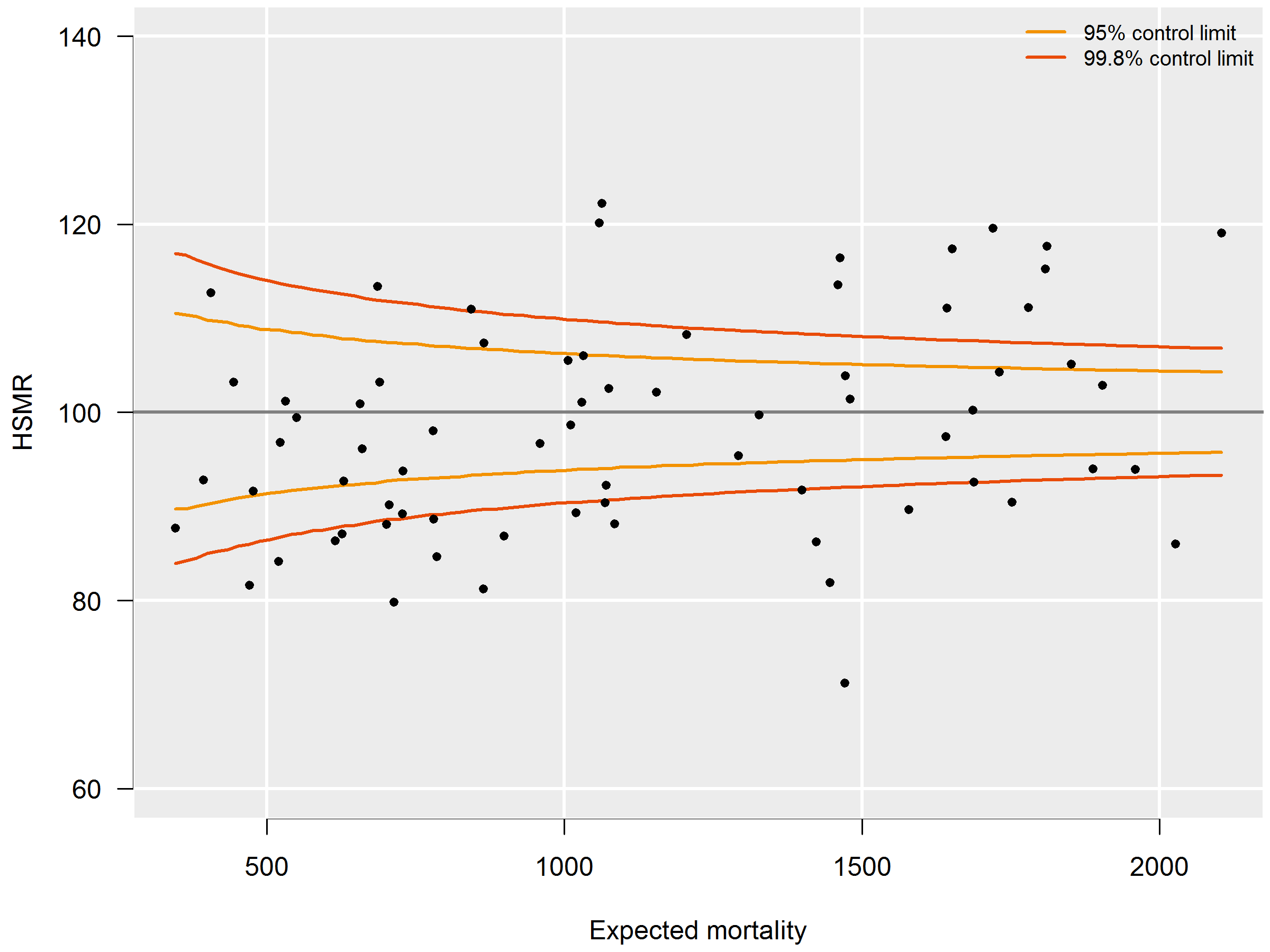
HSMRs can be presented in a funnel plot (see figure 3.6.4): a plot of hospitals, where the vertical axis represents the HSMRs and the horizontal axis the expected mortalities. Hospitals located above the horizontal axis (HSMR=100) have a higher than expected mortality. As this might be a non-significant feature based on chance, control limits are shown in the plot for each possible expected mortality. HSMRs within these control limits do not deviate significantly from 100. In the case of 95 percent control limits, about 2.5 percent of the points would be above the upper limit if there is no reason for differences between HSMRs, and about 2.5 percent of the points below the lower limit. The same holds, mutatis mutandis, for the 99.8 percent control limits. Here about 0.1 percent of the points would be located above the upper line if there is no reason for differences in standardised mortality rates. Most attention will be paid to this line, as points above this line have a high HSMR that is statistically very significant, which can hardly be the result of chance alone. These hospitals would be advised to investigate the possible reasons for the significantly high values: coding errors, unmeasured case mix variables and/or suboptimal quality of care.
The precision of the HSMR is much greater for a three-year period than for a single year, which is reflected by a smaller range between the control limits. The confidence intervals of the HSMR are also smaller. Of course, drawbacks are that two consecutive three-year figures (e.g. 2015-2017 and 2016-2018) overlap, and that the three-year figure is less up-to-date than the figure of the last year. Therefore we also calculated the HSMR figures for the most recent year. Observed mortality (numerator) and expected mortality (denominator) are then calculated for this year’s admissions, whereas the expected mortality model of the HSMR still uses the four-year data. If a hospital has a significantly high HSMR in the most recent year, but not in the three-year period, this is a signal for further investigation, as the quality of care may have deteriorated. There can also be other reasons for this, e.g. differences in registration practices over the years, but it is a signal for the hospital for further investigation.
On the other hand, if a hospital has a significantly high HSMR for the three-year period, but not in the last year, this does not necessarily mean that the situation has improved in the last year, as the one-year figures are less often significant because of the larger margins. In such cases, not only the significance should be taken into account, but also the HSMR levels over the years.
3.6.4 P-Values
From 2017 onwards, it was decided to also calculate p-values for the SMRs of the 158 diagnosis groups. The reason is that high SMRs for diagnosis groups are often an important starting point for further research and hospitals might need an extra tool for prioritizing such research, in case of multiple high SMRs. The lower the p-value, the more likely it is that the observed mortality deviates from the expected mortality. The p-values therefore allow hospitals to investigate their SMRs in order of significance (lowest p-values first). Also, because of the large number of diagnosis groups, there is a risk of incorrectly labelling SMRs as significantly high of low, i.e. the so called type I errors, or false-positives, due to multiple testing (Goeman and Solari, 2011). To reduce this risk, a lower p-value can be chosen as a cut-off. The p-values are not included in the reports sent to the hospitals, but hospitals can request them from Dutch Hospital Data.
Separate p-values are given for the alternative hypotheses: “the observed mortality (Odh) is higher than the expected mortality (Edh)” and “the observed mortality (Odh) is lower than the expected mortality (Edh).” The p-values belonging to the these hypotheses are denoted by Phigh (Odh) and Plow (Odh) respectively. The main reason for calculating two separate p-values is that by using a confidence of 99 percent for each of the two tests results in the same significant SMRs as found with the 98 percent confidence interval of the SMRs. Another reason is that often the main interest is Phigh (Odh).
The p-value of null-hypothesis “the observed mortality is lower or equal to the expected mortality” is given by the probability of observing a mortality equal to or higher than the observed mortality given the expected mortality:
\begin{equation}
p_\mathrm{high}(O_{dh}) = \Pr(X \ge O_{dh} | E_{dh}) = 1 - \Pr(X < O_{dh} | E_{dh})
\end{equation}
Assuming that the observed mortality follows a Poisson-distribution with and expected value equal to the expected mortality this is equal to
\begin{equation}
p_\mathrm{high}(O_{dh}) = 1-P_{E_{dh}}(X \le O_{dh}) + P_{E_{dh}}(X = O_{dh})
\end{equation}
With PEdh(X ≤ Odh) the cumulative distribution function and PEdh(X = Odh) the probability distribution function of the Poisson-distribution with an expected value of Edh.
Likewise the p-value of the null-hypothesis “the observed mortality is higher or equal to the expected mortality” is given by:
\begin{equation}
p_\mathrm{low}(O_{dh}) = P_{E_{dh}}(X \le O_{dh})
\end{equation}
2) For this criterion, all secondary diagnoses are considered, even if they do not belong to the 17 comorbidity groups used as covariates. If identical secondary diagnoses (identical ICD-10 codes) are registered within one admission, only one is counted. If a secondary diagnosis is identical to the main diagnosis of the admission, it is not counted as a secondary diagnosis.
4. Evaluation of the HSMR 2022 model
This chapter presents and evaluates the HSMR model results. Summary outcomes of the 158 logistic regressions are presented, with in-hospital mortality as the dependent variable and the variables mentioned in section 3.4 as explanatory variables. More detailed results are presented in the table “Statistical significance of covariates HSMR 2022 model” published together with this report. The regression coefficients and their standard errors are presented in the file “Coefficients HSMR 2022.xlsx”, published together with this report.
4.1 Target population and data set
All hospitals that register complete records of inpatient admissions and prolonged observations without overnight stay in the LBZ are included in the HSMR model. In 2019, 2020 and 2021 all general hospitals and university hospitals were included in the model, as well as three short-stay specialised hospitals (two cancer hospitals and an eye hospital). In 2022 a fourth short-stay specialised (orthopaedic) hospital registered admissions in the LBZ and was included in the model. All of the hospitals had completely registered all admissions in the LBZ.
The total number of hospitals included in the HSMR model of 2019-2022 is 75 and includes 64 general hospitals, 7 university hospitals and 4 short stay specialised hospitals. These numbers are based on the number of hospital units in 2022, counting hospitals that merged in 2022 as one unit for all years (2019-2022).
| 2019 | 2020 | 2021 | 2022 | total | |
|---|---|---|---|---|---|
| Excluded admissions not meeting the NZa criteria1) | 138,310 | 123,889 | 131,521 | 143,399 | 537,119 |
| Excluded admissions of foreigners | 9,825 | 6,231 | 5,993 | 7,973 | 30,022 |
| Excluded admissions due to COVID-192) | 40,430 | 60,228 | 100,658 | ||
| Excluded admissions of healthy persons3) | 19,151 | 18,202 | 19,196 | 18,943 | 75,492 |
| Total number of admissions included in model | 1,617,371 | 1,395,545 | 1,407,749 | 1,481,648 | 5,902,313 |
| Number of inpatient admissions | 1,504,130 | 1,288,291 | 1,295,255 | 1,367,700 | 5,455,376 |
| Number of observations | 113,241 | 107,254 | 112,494 | 113,948 | 446,937 |
| Number of deaths included in model | 32,647 | 29,151 | 29,779 | 36,207 | 127,784 |
| Crude mortality (in admissions in model) | 2.0% | 2.1% | 2.1% | 2.4% | 2.2% |
| 1) Admissions that do not meet the billing criteria of the Dutch Healthcare Authority (NZa) for inpatient admissions, and for prolonged observations, unplanned, without overnight stay. The number of these admissions in the LBZ varies over the years, due to different registration instructions of DHD. 2) Admissions with COVID-19 as the main diagnosis (ICD-10 codes U07.1 (COVID-19, virus identified (lab confirmed)), U07.2 (COVID-19, virus not identified (clinically diagnosed)) and, from 2021 onwards, U10.9 (Multisystem inflammatory syndrome associated with COVID-19, unspecified)). 3) Admissions of healthy persons are admissions of healthy newborns, healthy parents accompanying sick children, or other healthy boarders. | |||||
Table 4.1.1 lists some characteristics of the admissions included in the HSMR 2022 model per year. Admissions not meeting the criteria of the Dutch Healthcare Authority and admissions of foreigners were excluded. For the years 2020 and 2021, admissions with COVID-19 as the principal diagnosis were also excluded. In addition, from 2019 onwards, all admissions of healthy persons were excluded.
The number of admissions included in 2022 was 5% higher than in 2021, mostly due to the inclusion of admissions with COVID-19 as the principal diagnosis. However, the number of admissions was still 8% lower than in 2019, due to the ongoing overall impact of the COVID-19 pandemic on regular hospital care in 2022. The total number of admissions over all four years in the 2022 model was also 13% lower than in the 2019 model (6,777,534).
Crude mortality of the admissions included in the HSMR model was increased in 2022 compared to mortality of previous years. This was partly due to the inclusion of the COVID-19 admissions, that had had a much higher in-hospital mortality rate (10.0%, data not shown), but mortality of the non-COVID-19 admissions was also increased (2.3%, data not shown) in 2022.
The total number of admissions in the 2022 model (5,902,313; over all four years) was not only lower than in 2019, but was also 4% lower than in the 2021 model (6,124,777). This decrease is mostly due to the exclusion of the healthy persons: if those admissions had been included in the 2022 model, the number of admissions would have been only 2% lower when compared to that of the 2021 model. The additional decrease of 2% is probably due to the fact that the 2022 model is based on data of three pandemic years (2020-2022), while the 2021 model was based on data of two pandemic years (2020-2021) and two regular years (2018-2019).
4.2 Hospital exclusion
Hospitals were only provided with (H)SMR outcomes if the data fulfilled the criteria stated in paragraph 3.5. In order to qualify for a three-year report (2020-2022) hospitals had to fulfil these criteria for the three consecutive years.
Of the 75 hospitals included in the model, all had registered (valid) data over 2022. The four short stay specialised hospitals and one general hospital had not been asked to grant authorization for providing HSMR numbers because their case mix was very different from that of the other hospitals. In fact, all of these hospitals had participated in the LBZ but the data of these hospitals did not meet one or more of the previously stated criteria, such as a minimum number of 60 registered deaths or on average a minimum number of 0.5 comorbidities per admission. All of the other 70 hospitals that had granted authorization fulfilled the criteria and were provided with a HSMR figure for 2022. For these 70 hospitals the data of 2020 and 2021 was additionally investigated in order to determine if a three-year report could be provided. The data of all 70 hospitals met the criteria in all years considered and so all hospitals were also provided with three-year HSMR figures.
4.3 Impact of the covariates on mortality and HSMR
The table “Statistical significance of covariates HSMR 2022 model” published together with this report shows which covariates have a statistically significant (95 percent confidence) impact on in-hospital mortality for each of the 158 diagnosis groups: “1” indicates (statistical) significance, and “0” non-significance, while a dash (-) means that the covariate has been dropped as the number of admissions is smaller than 50 (or as there are no deaths) for all but one category of a covariate; see section 3.6.2.
The last row of the table “Statistical significance of covariates HSMR 2022 model” published together with this report gives the numbers of significant results across the diagnosis groups for each covariate. These values are presented again in table 4.3.1, as a summary, but ordered by the number of times a covariate is significant. As an additional model (COVID-19) was added this year, the numbers in the following tables have increased slightly compared to the previous year. Age, urgency of the admission, and severity of the main diagnosis are significant for a large majority of the diagnosis groups. This is also true for several of the comorbidity groups, especially for group 2 (Congestive heart failure and cardiomyopathy). Comorbidity 15 (HIV) is only rarely registered as a comorbidity; most diagnosis groups had fewer than 50 admissions with HIV comorbidity. In only one of the models comorbidity 15 was statistically significant. The number of times month of admission is significant varies over the years (CBS, 2018, 2019, 2020, 2021): it increased from 27 in 2017 to 43 in 2018, but in 2019 it decreased to 37, to 35 in 2020, to 33 in 2021 and to 28 in 2022. The number of times year of discharge is significant stabilized on 22 in the previous three HSMR models (CBS, 2020, 2021, 2022), but in the HSMR 2022 model it increased to 32, which was the largest increase of all covariates in the 2022 model. Compared to the HSMR 2021 model, other large changes were observed for the covariates comorbidity 3 (Peripheral vascular disease, significant in eight additional models) and comorbidity 12 (Hemiplegia or paraplegia, no longer significant in six models). The changes are smaller for the other covariates. The total number of significant covariates decreased from 1,632 in 2021 to 1,613 in 2022.
| Covariate | No. of significant results |
|---|---|
| Age | 140 |
| Urgency | 125 |
| Comorbidity 2 | 123 |
| Severity main diagnosis | 114 |
| Comorbidity 13 | 108 |
| Comorbidity 3 | 103 |
| Comorbidity 16 | 102 |
| Source of admission | 98 |
| Comorbidity 9 | 90 |
| Comorbidity 6 | 88 |
| Comorbidity 14 | 67 |
| Comorbidity 4 | 67 |
| Comorbidity 5 | 59 |
| Comorbidity 17 | 48 |
| Comorbidity 1 | 43 |
| Sex | 40 |
| Year of discharge | 32 |
| Comorbidity 10 | 30 |
| Month of admission | 28 |
| SES | 27 |
| Comorbidity 12 | 26 |
| Comorbidity 7 | 23 |
| Comorbidity 11 | 22 |
| Comorbidity 8 | 9 |
| Comorbidity 15 | 1 |
| Comorbidity groups: 1 Myocardial infarction, 2 Congestive heart failure and cardiomyopathy, 3 Peripheral vascular disease, 4 Cerebrovascular disease , 5 Dementia, 6 Pulmonary disease, 7 Connective tissue disorder, 8 Peptic ulcer, 9 Liver disease, 10 Diabetes, 11 Diabetes complications, 12 Hemiplegia or paraplegia, 13 Renal disease, 14 Cancer, 15 HIV, 16 Metastatic cancer, 17 Severe liver disease. | |
The significance only partially reflects the effect of the covariates on mortality. This is better measured using the Wald statistic. Table 4.3.2 presents the total of all Wald statistics summed over the diagnosis groups with the respective sum of the degrees of freedom, for each of the covariates ordered by value. It shows that severity of the main diagnosis has the highest explanatory power. Age and urgency of admission are also important variables. Of the comorbidities in the model, comorbidity groups 2, 16, and 13 are the groups with the most impact on mortality. Compared to the outcome of the 2021 model (CBS, 2022), the order of the covariates with regard to explanatory power is almost identical. Note that the values of the Wald statistics themselves cannot be compared directly between years as these values depend on the number of admissions used in the models.
| Covariate | Sum of Wald statistics | Sum of df |
|---|---|---|
| Severity main diagnosis | 38,786 | 401 |
| Age | 30,011 | 1,984 |
| Urgency | 16,237 | 155 |
| Comorbidity 2 | 9,356 | 146 |
| Comorbidity 16 | 4,210 | 140 |
| Comorbidity 13 | 3,605 | 151 |
| Source of admission | 2,984 | 283 |
| Comorbidity 3 | 2,468 | 147 |
| Comorbidity 6 | 2,085 | 152 |
| Comorbidity 9 | 1,762 | 125 |
| Month of admission | 1,535 | 790 |
| Comorbidity 17 | 1,451 | 64 |
| Comorbidity 4 | 1,293 | 123 |
| Comorbidity 14 | 1,263 | 143 |
| Comorbidity 5 | 1,221 | 120 |
| SES | 1,023 | 696 |
| Year of discharge | 884 | 469 |
| Sex | 773 | 149 |
| Comorbidity 12 | 753 | 98 |
| Comorbidity 1 | 638 | 149 |
| Comorbidity 10 | 428 | 153 |
| Comorbidity 11 | 328 | 117 |
| Comorbidity 7 | 298 | 130 |
| Comorbidity 8 | 114 | 32 |
| Comorbidity 15 | 18 | 12 |
| Comorbidity groups: 1 Myocardial infarction, 2 Congestive heart failure and cardiomyopathy, 3 Peripheral vascular disease, 4 Cerebrovascular disease , 5 Dementia, 6 Pulmonary disease, 7 Connective tissue disorder, 8 Peptic ulcer, 9 Liver disease, 10 Diabetes, 11 Diabetes complications, 12 Hemiplegia or paraplegia, 13 Renal disease, 14 Cancer, 15 HIV, 16 Metastatic cancer, 17 Severe liver disease. | ||
The explanatory power of year of discharge stabilized in the HSMR 2019 and HSMR 2020 models, increased slightly (+5%) in the HSMR 2021 model and shows a further increase of 13% in the HSMR 2022 model. This implies that the differences in mortality between the years in the model (corrected for differences in patient characteristics) has slightly increased, probably because of the influence of the COVID-19 pandemic on an increasing number of years in the model and the higher mortality of non-COVID-19 admissions in 2022.
Similar to previous years, the impact of comorbidity 1 (myocardial infarction) is decreasing, with a 45% decrease over the past seven models. In addition, the impact of comorbidity 14 (cancer) has decreased by 31% since the 2016 model. A decreased impact of a comorbidity could reflect a decreased effect of the comorbidity (e.g. the likelihood of dying in hospital when having this condition as comorbidity has decreased), and/or a decreased number of patients with this comorbidity resulting in less accurate estimates of the effect of this comorbidity (which also decreases the Wald statistic). The opposite applies in the case of an increased impact of a variable.
The impact of the SES variable was relatively stable up to the 2020 model. In the 2021 model the explanatory power of SES increased by 12%, and the HSMR 2022 model shows a further increase of 10%. In total the impact of SES has increased by 23% compared to the 2020 model. This is probably a result of the use of updated values of the SES variable on the data of 2021 in the HSMR 2021 model and on the data of all years (2019-2022) in the 2022 model (see section 2.2 for more details on the update of the SES variable).
In addition, the impact of month of admission has also increased in the 2022 model (1,535) compared to the 2021 model (1,375). This is due to the inclusion of COVID-19 in the 2022 model, as month of admission is the second most important covariate in the COVID-19 model with a Wald of 270. This is probably caused by the monthly variation in the number of COVID-19 admissions and/or the likelihood of in-hospital mortality, which are in turn affected by the COVID-19 transmission waves in the population (four waves in 2022). During the influenza epidemic in 2018, the impact of month of admission was also increased compared to previous and consecutive models.
As was mentioned in section 3.6.2, when the hospitals differ little on a covariate, the effect of this covariate on the HSMR can still be small even if this covariate is a strong predictor for mortality. Table 4.3.3 shows the impact of each covariate on the HSMR, as measured by the formula in paragraph 3.6.2, for the hospitals for which HSMRs are calculated. The comorbidities, which are considered here as one group (17 comorbidities together), have the largest effect on the HSMR. This is caused by differences in case mixes between hospitals, but possibly also by differences in coding practices (see Van der Laan, 2013). Deleting sex as a covariate hardly has an impact on the HSMRs, whereas SES has a reasonable impact on the HSMR. This is probably because hospitals differ more in terms of SES categories of the postal areas in their vicinity than in terms of the sex distribution of their patients. In the HSMR 2022 model, the impact of SES increased compared to the 2021 model and now exceeds that of source of admission. For the other covariates in table 4.3.3 the order (ranked by magnitude of the effect) is the same as in the previous model.
| Covariate | Average shift in HSMR |
|---|---|
| Comorbidity1) | 4.52 |
| Age | 3.75 |
| Severity main diagnosis | 2.40 |
| Urgency | 1.95 |
| SES | 1.03 |
| Source of admission | 0.98 |
| Month of admission | 0.20 |
| Sex | 0.11 |
| 1) The comorbidities were deleted as one group and not separately. | |
4.4 Model evaluation for the 158 regression analyses
Table 4.4.1 presents numbers of admissions and deaths, and C-statistics for the 158 diagnosis groups. The C-statistic is explained in section 3.6.2. Overall the C-statistics have changed little compared to the previous model. Only two C-statistics showed a moderate change: after last year’s increase from 0.94 to 0.98, the C-statistic of “Cancer of testis and other male genital organs” decreased to 0.94. In addition, the C-statistic of “Other and unspecified benign neoplasm” decreased from 0.88 to 0.84. All other changes are smaller than 0.04 with most of them below 0.02. For 66 diagnosis groups the C-statistic did not change compared to last year.
Only three of the 158 diagnosis groups have a C-statistic below 0.70: “Congestive heart failure, nonhypertensive” (70), “Chronic obstructive pulmonary disease and bronchiectasis” (82) and “Aspiration pneumonitis; food/vomitus” (84). For the diagnosis groups with a C-statistic below 0.7, the model’s ability to explain patient mortality is less than ‘good’. This increases the risk that the model does not completely correct for population differences between the hospitals. For the highest scoring diagnosis groups (above 0.9) the covariates strongly reduce the uncertainty in predicting patient mortality. In 2022, 56 diagnosis groups had a C-statistic above 0.9.
As mentioned in section 2.2, admissions of healthy persons (such as healthy newborns and other healthy boarders) are excluded in the present HSMR model. The large majority of these admissions were formerly part of diagnosis groups 157 (“Residual codes: unclassified”) and group 118 (”Complications of pregnancy, childbirth, and the puerperium; liveborn”). Smaller numbers of these admissions were previously part of diagnosis groups 131 (“Other perinatal conditions”) and 130 (“Intrauterine hypoxia, perinatal asphyxia, and jaundice”) mainly. The C-statistics of these four groups have not changed much in the HSMR 2022 model compared to the 2021 model (resp. -0.021, 0.018, 0.005 and 0.004). Therefore, excluding the admissions of healthy persons did not affect the ability of the models to predict mortality.
| Diag. group no. | Description of diagnosis group | Number of admissions | Number of deaths | C-statistic |
|---|---|---|---|---|
| 1 | Tuberculosis | 1,468 | 45 | 0.88 |
| 2 | Septicemia (except in labor) | 12,320 | 3,490 | 0.73 |
| 3 | Bacterial infection, unspecified site | 9,796 | 606 | 0.80 |
| 4 | Mycoses | 2,458 | 277 | 0.79 |
| 5 | HIV infection | 717 | 26 | 0.83 |
| 6 | Hepatitis, viral and other infections | 23,571 | 272 | 0.93 |
| 7 | Cancer of head and neck | 14,785 | 241 | 0.90 |
| 8 | Cancer of esophagus | 10,350 | 593 | 0.79 |
| 9 | Cancer of stomach | 11,267 | 439 | 0.82 |
| 10 | Cancer of colon | 42,673 | 1,125 | 0.84 |
| 11 | Cancer of rectum and anus | 17,669 | 384 | 0.86 |
| 12 | Cancer of liver and intrahepatic bile duct | 7,499 | 433 | 0.82 |
| 13 | Cancer of pancreas | 17,295 | 906 | 0.82 |
| 14 | Cancer of other GI organs, peritoneum | 8,673 | 390 | 0.79 |
| 15 | Cancer of bronchus, lung | 50,474 | 4,224 | 0.81 |
| 16 | Cancer, other respiratory and intrathoracic | 2,333 | 130 | 0.85 |
| 17 | Cancer of bone and connective tissue | 8,227 | 97 | 0.91 |
| 18 | Melanomas of skin and other non-epithelial cancer of skin | 6,314 | 108 | 0.93 |
| 19 | Cancer of breast | 39,216 | 375 | 0.97 |
| 20 | Cancer of uterus | 9,044 | 127 | 0.93 |
| 21 | Cancer of cervix and other female genital organs | 10,597 | 93 | 0.94 |
| 22 | Cancer of ovary | 8,221 | 253 | 0.85 |
| 23 | Cancer of prostate | 25,490 | 350 | 0.94 |
| 24 | Cancer of testis and other male genital organs | 6,461 | 6 | 0.94 |
| 25 | Cancer of bladder | 53,975 | 444 | 0.93 |
| 26 | Cancer of kidney, renal pelvis and other urinary organs | 15,649 | 271 | 0.88 |
| 27 | Cancer of brain and nervous system | 11,955 | 264 | 0.79 |
| 28 | Cancer of thyroid | 5,955 | 51 | 0.98 |
| 29 | Hodgkin`s disease | 1,880 | 41 | 0.91 |
| 30 | Non-Hodgkin`s lymphoma | 22,724 | 964 | 0.83 |
| 31 | Leukemias | 21,515 | 1,211 | 0.80 |
| 32 | Multiple myeloma | 10,378 | 456 | 0.79 |
| 33 | Cancer, other and unspec. primary, maintenance chemotherapy and radioth. | 4,701 | 116 | 0.90 |
| 34 | Secondary malignancies | 79,076 | 4,245 | 0.77 |
| 35 | Malignant neoplasm without specification of site | 2,386 | 314 | 0.82 |
| 36 | Neoplasms of unspecified nature or uncertain behavior | 11,410 | 216 | 0.89 |
| 37 | Other and unspecified benign neoplasm | 64,352 | 94 | 0.84 |
| 38 | Thyroid and other endocrine disorders | 23,092 | 220 | 0.91 |
| 39 | Diabetes mellitus without complication | 13,509 | 127 | 0.87 |
| 40 | Diabetes mellitus with complications | 23,510 | 504 | 0.85 |
| 41 | Nutritional deficiencies and other nutritional, endocrine, and metabolic disorders | 56,770 | 473 | 0.95 |
| 42 | Fluid and electrolyte disorders | 33,116 | 896 | 0.85 |
| 43 | Cystic fibrosis | 1,900 | 5 | 0.88 |
| 44 | Immunity and coagulation disorders, hemorrhagic disorders | 10,607 | 176 | 0.87 |
| 45 | Deficiency and other anemia | 48,015 | 483 | 0.80 |
| 46 | Diseases of white blood cells | 8,832 | 233 | 0.75 |
| 47 | Mental, affective, anxiety, somatoform, dissociative, and personality disorders | 20,370 | 70 | 0.88 |
| 48 | Senility and organic mental disorders | 10,093 | 535 | 0.71 |
| 49 | Schizophrenia, mental retardation, preadult disorders and other mental cond. | 6,209 | 20 | 0.95 |
| 50 | Other psychoses | 2,763 | 27 | 0.86 |
| 51 | Meningitis, encephalitis, and other central nervous system infections | 9,162 | 530 | 0.87 |
| 52 | Parkinson`s disease | 5,182 | 90 | 0.84 |
| 53 | Multiple sclerosis and other degenerative nervous system conditions | 11,544 | 276 | 0.91 |
| 54 | Paralysis and late effects of cerebrovascular disease | 3,633 | 60 | 0.86 |
| 55 | Epilepsy and convulsions | 42,846 | 587 | 0.88 |
| 56 | Coma, stupor, and brain damage | 2,106 | 201 | 0.90 |
| 57 | Headache and other disorders of the sense organs | 59,246 | 43 | 0.93 |
| 58 | Other nervous system disorders | 52,313 | 352 | 0.94 |
| 59 | Heart valve disorders | 36,128 | 823 | 0.77 |
| 60 | Peri-, endo-, myocarditis, and cardiomyopathy | 21,619 | 669 | 0.87 |
| 61 | Essential hypertension, hypertension with compl., and secondary hypertension | 12,750 | 106 | 0.93 |
| 62 | Acute myocardial infarction | 136,759 | 3,399 | 0.85 |
| 63 | Coronary atherosclerosis and other heart disease | 104,278 | 766 | 0.85 |
| 64 | Nonspecific chest pain | 143,800 | 32 | 0.92 |
| 65 | Pulmonary heart disease | 30,819 | 1,043 | 0.80 |
| 66 | Other and ill-defined heart disease | 1,393 | 111 | 0.88 |
| 67 | Conduction disorders (heart disease) | 24,903 | 367 | 0.88 |
| 68 | Cardiac dysrhythmias | 175,085 | 770 | 0.90 |
| 69 | Cardiac arrest and ventricular fibrillation | 15,662 | 5,746 | 0.75 |
| 70 | Congestive heart failure, nonhypertensive | 126,149 | 9,986 | 0.67 |
| 71 | Acute cerebrovascular disease | 153,889 | 12,959 | 0.80 |
| 72 | Transient cerebral ischemia, and other cerebrovascular disease | 43,625 | 322 | 0.90 |
| 73 | Peripheral and visceral atherosclerosis | 45,661 | 1,924 | 0.91 |
| 74 | Aortic and other artery aneurysms | 27,019 | 2,446 | 0.89 |
| 75 | Aortic and arterial embolism or thrombosis | 11,114 | 444 | 0.85 |
| 76 | Other circulatory disease | 29,355 | 560 | 0.87 |
| 77 | Phlebitis, varicose veins, and hemorrhoids | 10,564 | 144 | 0.87 |
| 78 | Pneumonia | 107,767 | 9,095 | 0.75 |
| 79 | Influenza | 17,286 | 772 | 0.80 |
| 80 | Tonsillitis and upper respiratory infections | 49,684 | 88 | 0.92 |
| 81 | Acute bronchitis | 26,597 | 63 | 0.94 |
| 82 | Chronic obstructive pulmonary disease and bronchiectasis | 102,757 | 6,293 | 0.69 |
| 83 | Asthma | 23,518 | 96 | 0.91 |
| 84 | Aspiration pneumonitis, food/vomitus | 8,307 | 1,710 | 0.64 |
| 85 | Pleurisy, pneumothorax, pulmonary collapse | 22,286 | 613 | 0.83 |
| 86 | Respiratory failure, insufficiency, arrest | 5,346 | 1,629 | 0.74 |
| 87 | Lung disease due to external agents | 1,749 | 163 | 0.77 |
| 88 | Other lower respiratory disease | 24,230 | 997 | 0.87 |
| 89 | Other upper respiratory disease | 49,188 | 303 | 0.90 |
| 90 | Intestinal infection | 44,894 | 542 | 0.89 |
| 91 | Disorders of mouth, teeth, and jaw | 20,399 | 56 | 0.96 |
| 92 | Esophageal disorders | 12,162 | 115 | 0.91 |
| 93 | Gastroduodenal ulcer | 4,974 | 233 | 0.92 |
| 94 | Gastritis, duodenitis, and other disorders of stomach and duodenum | 7,312 | 85 | 0.87 |
| 95 | Appendicitis and other appendiceal conditions | 70,092 | 77 | 0.96 |
| 96 | Peritonitis and intestinal abscess | 5,125 | 359 | 0.80 |
| 97 | Abdominal hernia | 43,306 | 458 | 0.91 |
| 98 | Regional enteritis and ulcerative colitis | 17,343 | 63 | 0.95 |
| 99 | Intestinal obstruction without hernia | 33,245 | 1,509 | 0.82 |
| 100 | Diverticulosis and diverticulitis | 35,204 | 506 | 0.92 |
| 101 | Anal and rectal conditions | 21,761 | 50 | 0.94 |
| 102 | Biliary tract disease | 112,762 | 1,045 | 0.90 |
| 103 | Liver disease, alcohol-related | 7,345 | 918 | 0.72 |
| 104 | Other liver diseases | 17,814 | 1,058 | 0.82 |
| 105 | Pancreatic disorders (not diabetes) | 36,230 | 843 | 0.84 |
| 106 | Gastrointestinal hemorrhage | 36,590 | 1,066 | 0.80 |
| 107 | Noninfectious gastroenteritis | 11,105 | 218 | 0.80 |
| 108 | Other gastrointestinal disorders | 34,255 | 774 | 0.94 |
| 109 | Nephritis, nephrosis, renal sclerosis | 14,506 | 110 | 0.91 |
| 110 | Acute and unspecified renal failure | 15,123 | 998 | 0.76 |
| 111 | Chronic kidney disease | 13,475 | 457 | 0.87 |
| 112 | Urinary tract infections | 96,727 | 2,773 | 0.77 |
| 113 | Calculus and other diseases of urinary tract | 79,823 | 185 | 0.91 |
| 114 | Genitourinary symptoms and ill-defined conditions | 25,847 | 118 | 0.87 |
| 115 | Hyperplasia of prostate and other male genital disorders | 41,436 | 49 | 0.92 |
| 116 | Non-neoplastic breast conditions | 12,900 | 4 | 0.98 |
| 117 | Prolapse and other female genital disorders | 59,737 | 36 | 0.98 |
| 118 | Complications of pregnancy, childbirth, and the puerperium, liveborn | 545,091 | 16 | 0.86 |
| 119 | Skin and subcutaneous tissue infections | 52,885 | 786 | 0.89 |
| 120 | Other skin disorders, chronic ulcer of skin | 16,794 | 232 | 0.92 |
| 121 | Infective arthritis and osteomyelitis | 13,713 | 309 | 0.89 |
| 122 | Osteoarthritis, rheumatoid arthritis, and other musculoskeletal deformities | 227,38 | 183 | 0.93 |
| 123 | Other non-traumatic joint disorders | 10,528 | 35 | 0.92 |
| 124 | Spondylosis, back problems, and osteoporosis | 81,722 | 191 | 0.96 |
| 125 | Pathological fracture | 5,075 | 73 | 0.83 |
| 126 | Other connective tissue disease | 31,263 | 304 | 0.97 |
| 127 | Cardiac and circulatory congenital anomalies | 8,937 | 167 | 0.89 |
| 128 | Noncardiac congenital anomalies | 26,163 | 199 | 0.95 |
| 129 | Short gestation, low birth weight, and fetal growth retardation | 76,243 | 469 | 0.88 |
| 130 | Intrauterine hypoxia, perinatal asphyxia, and jaundice | 61,417 | 213 | 0.95 |
| 131 | Other perinatal conditions | 225,501 | 215 | 0.95 |
| 132 | Joint disorders and dislocations, trauma-related, sprains and strains | 20,737 | 30 | 0.98 |
| 133 | Fracture of neck of femur (hip) | 87,646 | 2,729 | 0.80 |
| 134 | Skull and face fractures, spinal cord injury | 11,339 | 196 | 0.90 |
| 135 | Fracture of upper limb | 41,769 | 133 | 0.95 |
| 136 | Fracture of lower limb | 49,742 | 288 | 0.94 |
| 137 | Other fractures | 43,858 | 1,032 | 0.85 |
| 138 | Intracranial injury | 39,463 | 2,699 | 0.77 |
| 139 | Crushing injury or internal injury | 20,300 | 437 | 0.91 |
| 140 | Open wounds of head, neck, and trunk | 5,595 | 46 | 0.87 |
| 141 | Open wounds of extremities | 5,124 | 37 | 0.95 |
| 142 | Complication of device, implant or graft | 96,699 | 1,336 | 0.88 |
| 143 | Complications of surgical procedures or medical care | 98,780 | 848 | 0.86 |
| 144 | Superficial injury, contusion | 58,104 | 475 | 0.92 |
| 145 | Burns | 3,743 | 85 | 0.92 |
| 146 | Poisoning by psychotropic agents, drugs, or other medications | 36,244 | 348 | 0.85 |
| 147 | Other injuries and conditions due to external causes | 13,360 | 685 | 0.89 |
| 148 | Syncope | 42,043 | 126 | 0.84 |
| 149 | Fever of other and unknown origin | 19,215 | 101 | 0.82 |
| 150 | Lymphadenitis and gangrene | 3,883 | 21 | 0.97 |
| 151 | Shock | 1,273 | 480 | 0.74 |
| 152 | Nausea and vomiting | 11,529 | 70 | 0.85 |
| 153 | Abdominal pain | 37,891 | 111 | 0.95 |
| 154 | Malaise and fatigue | 8,820 | 143 | 0.82 |
| 155 | Allergic reactions | 10,868 | 34 | 0.96 |
| 156 | Rehabilitation and other aftercare, medical examination/ evaluation/screening | 75,286 | 219 | 0.85 |
| 157 | Residual codes, unclassified | 29,831 | 151 | 0.96 |
| 158 | COVID-19 | 27,988 | 2,803 | 0.75 |
4.5 Evaluation of the COVID-19 model
As this is the first year for which admissions with main diagnosis COVID-19 are included in the HSMR, this section will specifically describe the COVID-19 model. Last year (CBS, 2022), a separate model for COVID-19 was estimated but the COVID-19 admissions were not included in the HSMR of 2021. The previous COVID-19 model was estimated using data from 2021. The current model is estimated using data from 2022.
The current model has a C-statistic of 0.748. Although this is lower than the value 0.803 that was found for 2021, a C-statistic of 0.748 is still good. Between 2021 and 2022 there have been a number of changes in the data and admissions that might explain the difference in C-statistic.
First, the amount of COVID-19 admissions has dropped from 60,228 to 27,988 and the crude mortality rate has dropped from 14% to 10%. Higher levels of acquired immunity (by vaccination or earlier exposure to COVID-19) in 2022 may be one of the factors that can have contributed to this.
Second, we see that some of the effects of the covariates have changed. Table 4.5.1 shows the Wald statistics and the statistical significance for each of the covariates in the current model.
Age is still the most important predictor. However, where age explained approximately 75 percent of the variance in 2021, it explains about 50 percent in 2022. In 2022 a higher percentage of the COVID-19 admissions were in the age group >70 years and these admissions had considerably lower mortality than in 2021. Also there were more COVID-19 admissions of children in 2022, with almost zero mortality in both years. In the age-group 40-70 there were relatively less admissions in 2022, with a slightly higher mortality. Compared to 2021 the covariate ‘month of admission’ has become more important. Especially in the first months of 2022 the number of admissions was relatively high. The crude mortality rate was also somewhat higher in these months. Furthermore, there were four distinct COVID-19 admission waves in 2022 while in 2021 the number of monthly admissions was more constantly high. There are also some differences in other covariates. For example, with regard to the covariate ‘source of admission’ there were less admissions with source of admission equal to ‘other hospital’ in 2022 than in 2021. This is probably due to the fact that in 2022 there were less transfers of COVID-19 patients between hospitals.
All in all there have been several significant changes in the patient and admission characteristics in 2022 compared to 2021. The net result is that predicting mortality has become somewhat more difficult in 2022 for the COVID-19 admissions.
| Covariate | Wald | Significant |
|---|---|---|
| Age | 952 | 1 |
| Month of admission | 270 | 1 |
| Comorbidity 2 | 124 | 1 |
| Comorbidity 13 | 71 | 1 |
| Source of admission | 70 | 1 |
| Comorbidity 14 | 68 | 1 |
| Sex | 40 | 1 |
| Comorbidity 3 | 28 | 1 |
| Severity diagnosis | 21 | 1 |
| Comorbidity 7 | 19 | 1 |
| Comorbidity 17 | 13 | 1 |
| Comorbidity 9 | 12 | 1 |
| Comorbidity 12 | 11 | 1 |
| SES | 5 | 0 |
| Comorbidity 4 | 5 | 1 |
| Comorbidity 6 | 5 | 1 |
| Urgency | 3 | 0 |
| Comorbidity 11 | 3 | 0 |
| Comorbidity 16 | 3 | 0 |
| Comorbidity 1 | 2 | 0 |
| Comorbidity 5 | 1 | 0 |
| Comorbidity 10 | 0 | 0 |
| Comorbidity 8 | - | - |
| Comorbidity 15 | - | - |
The HSMR figures based on the model of 2021 did not include the COVID-19 admissions, whereas the current HSMR does, but only for the year 2022. To assess the impact of including the COVID-19 admissions in the HSMR 2022, we calculated the change in the HSMR outcomes with and without COVID-19. On average the HSMR for 2022 changes by 1.1 points (mean absolute difference between the HSMR of 2022 and that without including COVID-19), so removing the COVID-19 admissions has a small effect on the HSMR 2022. As the COVID-19 admissions are only included for 2022, the effect of removing COVID-19 admissions on the total HSMR for the three-year period 2020-2022 is smaller: 0.4 points. Figure 4.5.2 shows the change in the HSMR of 2022 for the individual hospitals. For most hospitals the change is smaller than 2 points. The maximum difference is 3.4 points.
| diff2022_cat | n (Number of hospitals) |
|---|---|
| -4 to -3 | 1 |
| -3 to -2 | 2 |
| -2 to -1 | 14 |
| -1 to 0 | 21 |
| 0 to 1 | 15 |
| 1 to 2 | 14 |
| 2 to 3 | 2 |
| 3 to 4 | 1 |
As shown in table 4.5.3, there are three hospitals that change from a significantly low HSMR 2022 to a non-significant HSMR 2022, or vice versa, when removing COVID-19 admissions. For the HSMR of 2020-2022, the HSMR of only two hospitals change from significantly low or high to non-significant (table 4.5.4). A comparison of HSMRs with and without COVID-19 admissions was also described in the methodological report of the HSMR 2021 (CBS, 2022) and showed larger differences (with 8 hospitals changing in significance categories). Thus the impact of in or excluding COVID-19 admissions on the HSMRs has decreased in 2022, which may be due to the lower number of COVID-19 admissions in 2022 and possibly the treatment of COVID-19 has also become more integrated in regular hospital care.
| HSMR 2022 without COVID-19 | |||
|---|---|---|---|
| HSMR 2022 | Low | Not-significant | High |
| Low | 12 | 2 | 0 |
| Not-significant | 1 | 45 | 0 |
| High | 0 | 0 | 10 |
| HSMR 2020-2022 without COVID-19 | |||
|---|---|---|---|
| HSMR 2020-2022 | Low | Not-significant | High |
| Low | 19 | 1 | 0 |
| Not-significant | 0 | 37 | 0 |
| High | 0 | 1 | 12 |
4.6 Regression coefficients
The file “coefficients HSMR 2022.xls” contains the estimated regression coefficients (columns “Estimate”), also called “log-odds”, for each of the 158 logistic regressions, as well as their standard errors (columns “Std. Err.”). The estimated regression coefficients are the elements of the estimate of vector 𝛽d in the formula for p̂dhi (see section 3.6.1), for each diagnosis d. Notice that a β-coefficient has to be interpreted as the difference in log-odds between the category in question and the reference category (first category of the same covariate). For the sake of clarity, the reference categories are given in the first row of the corresponding covariates and these have by definition a zero coefficient for each regression.
In many cases categories are collapsed (see section 3.6.2). This results in equal coefficients for the collapsed categories. If all categories were collapsed into one category for a certain variable and for a certain diagnosis group (i.e. if there was only one category with ≥50 admissions and ≥1 death), the variable was dropped from the model and all associated coefficients were set to zero. Therefore, the coefficients in the file “coefficients HSMR 2022.xls” can be used directly to calculate mortality probabilities, with the exception of two of the Charlson comorbidities (Comorbidity 17 and Comorbidity 11). If Charlson comorbidity 17 (Severe liver disease) contains <50 admissions or no mortality, it is collapsed with Charlson comorbidity 9 (Liver disease). In this case the coefficient of Comorbidity 17 is set to zero. When a patient has both comorbidities, it counts as only one comorbidity. Therefore, when the coefficient of Comorbidity 17 is zero in the coefficients file, one should first recode all Charlson 17 comorbidities to Comorbidity 9 and use the coefficient of Comorbidity 9. The same holds for Charlson 11 (Diabetes complications) when it is collapsed with Charlson 10 (Diabetes).
5. Conclusions
Compared to the HSMR model of previous year the largest change in the present HSMR model of 2019-2022 is that the COVID-19 admissions have been included (for 2022). Smaller changes are the exclusion of admissions of healthy persons (e.g. healthy newborns and other healthy boarders), and the application of the new variable for socioeconomic status (SES) to all model years. In the model of previous year the new SES variable was applied to the 2021 data only.
Sections 4.4 and 4.5 evaluate the quality of the present HSMR model. The results are largely comparable to the models of previous years. Overall the C-statistics have changed little compared to the previous model. The order of the covariates with regard to explanatory power is mostly the same, although some minor changes have occurred in the relative importance of some of the variables. Year of discharge and month of admission have become somewhat more important, which is probably caused by larger swings in mortality caused by effects of the different waves of the COVID-19 pandemic over the years. The explanatory power of SES has also increased, which is most likely due to the implementation of the new SES variable.
The effect of including the COVID-19 admissions on the total HSMR of 2022 is relatively small – for most hospitals the effect is less than 2 points. The 2022 model for the COVID-19 admissions has somewhat more difficulty predicting mortality than the COVID-19 model of 2021 (which was not included in the HSMR 2021). This is probably due to the changes in patient and admission characteristics of the COVID-19 admissions in 2022 compared to 2021. The predictive power of the COVID-19 model of 2022 is however still good and comparable to the models for other diagnoses.
6. References
Arts, K., R. van Gaalen, J. van der Laan, F. Linder, J. Mol, J. van Rooijen and C. Siermann (2022). Berekenwijze Sociaal Economische Status scores, Statistics Netherlands, The Hague/Heerlen.
Bottle, A., B. Jarman and P. Aylin (2011). Hospital standardized mortality ratios: sensitivity analyses on the impact of coding. Health Serv Res 46(6 Pt 1):1741–61.
Campbell, M.J., R.M. Jacques, J. Fotheringham, T. Pearson, R. Maheswaran and J. Nicholl (2011). An evaluation of the Summary Hospital Mortality Index, final report. School of Health and Related Research, The University of Sheffield.
CBS (2011, 2012, 2013,… etc.). HSMR 2010 [2011, 2012, …etc.], Methodological report. Statistics Netherlands, The Hague/Heerlen.
Cecil, E., A. Bottle, A. Esmail, C. Vincent and P. Aylin (2020). What is the relationship between mortality alerts and other indicators of quality of care? A national cross-sectional study. Journal of Health Services Research & Policy 25(1): 13-21.
Chong, C.A.K.Y., G.C. Nguyen and M.E. Wilcox (2012). Trends in Canadian hospital standardised mortality ratios and palliative care coding 2004-2010: a retrospective database analyses.. BMJ Open 2012;2:e001729. doi:10.1136/bmjopen-2012-001729.
Goeman, J.J. and A. Solari (2011). Multiple Testing for Exploratory Research. Statist. Sci. 26 (4), November 2011. https://doi.org/10.1214/11-STS356, 584-597.
Haas, E.J., F.J. Angulo, J.M. McLaughlin, E. Anis, S.R. Singer, F. Khan, ... & S. Alroy-Preis (2021). Impact and effectiveness of mRNA BNT162b2 vaccine against SARS-CoV-2 infections and COVID-19 cases, hospitalisations, and deaths following a nationwide vaccination campaign in Israel: an observational study using national surveillance data. The Lancet, 397(10287), 1819-1829.
Heijink, R., X. Koolman, D. Pieter, A. van der Veen, B. Jarman and G. Westert (2008). Measuring and explaining mortality in Dutch hospitals; The Hospital Standardized Mortality Rate between 2003 and 2005. BMC Health Services Research 8:73.
HSCIC (2016). Indicator Specification: Summary Hospital-level Mortality Indicator. Version 1.22, 24 February 2016. Health & Social Care Information Centre.
Jarman, B., D. Pieter, A.A. van der Veen, R.B. Kool, P. Aylin, A. Bottle and G.P. Westert (2010). The hospital standardised mortality ratio: a powerful tool for Dutch hospitals to assess their quality of care? Qual Saf Healthcare 19, 9-13.
Jarman, B., S. Gault, B. Alves, A. Hider, S. Dolan, A. Cook, B. Hurwitz and L.I. Iezzoni (1999). Explaining differences in English hospital death rates using routinely collected data, BMJ 318, 1515-1519.
Lamarche-Vadel, A., M. Ngantcha, M.-A. Le Pogamm, C. Grenier, L. Meyer and G. Rey (2015). Hospital comparisons based on mortality: revisiting the choice of postadmission timeframe and evaluating the contribution of cause-of-death data, France, 2009. Medical Care 53, 736-742.
Lilford, R. and P. Pronovost (2010). Using hospital mortality rates to judge hospital performance: a bad idea that just won’t go away. BMJ 340:c2016.
Mitchell, T.M. (2016). “Estimating Probabilities” additional chapter for the book Mitchell, T.M. (1997). Machine Learning. McGraw-Hill, New York.
NHS - The Health and Social Care Information Centre (2013). The use of palliative care coding in the Summary Hospital-level Mortality Indicator.
Ploemacher, J, A.Z. Israëls, D.J. van der Laan and A. de Bruin (2013). Gestandaardiseerde ziekenhuissterfte daalt in de tijd. Ned Tijdschr Geneeskd. 157 (22), 1034-1039.
Pouw, M.E., L.M. Peelen, K.G.M. Moons, C.J. Kalkman and H.F. Lingsma (2013). Including post-discharge mortality in the calculation of hospital standardised mortality ratios: a retrospective analysis of hospital episode statistics. BMJ 347:f5913.
Prismant (2008). De toepasbaarheid van de HSMR in het toezicht van de inspectie voor de gezondheidszorg. Prismant, Utrecht.
Quan H, V. Sundararajan, P. Halfon, A. Fong A, B. Burnand, J.C. Luthi, L.D. Saunders, C.A. Beck, T. E. Feasby, W.A. Ghali (2005). Coding algorithms for defining comorbidities in ICD-9-CM and ICD-10 administrative data. Medical Care 43, 1130-1139.
R Core Team (2015). R: A language and environment for statistical computing. R Foundation for Statistical Computing, Vienna, Austria.
RIVM and CBS (2022). Sterfte en oversterfte in 2020 en 2021: Onderzoek door het CBS en het RIVM, in het kader van het ZonMw onderzoeksprogramma Oversterfte. National Institute for Public Health and the Environment (RIVM), Bilthoven, and Statistics Netherlands (CBS), The Hague/Heerlen.
Van den Bosch, W.F., J. Silberbusch, K.J. Roozendaal and C. Wagner (2010). Variatie in codering patiëntengegevens beïnvloedt gestandaardiseerd ziekenhuissterftecijfer. Ned Tijdschr Geneeskd. 154 (2), 1-9.
Van den Bosch, W.F., P. Spreeuwenberg and C. Wagner (2011). Gestandaardiseerd ziekenhuissterftecijfer (HSMR): correctie voor ernst hoofddiagnose kan beter. Ned Tijdschr Geneeskd. 155:A3299, 66-75.
Van der Laan, D.J. (2013). Quality of the Dutch Medical Registration (LMR) for the calculation of the Hospital Standardised Mortality Ratio. Statistics Netherlands, The Hague/Heerlen.
Van der Laan, D.J., A. de Bruin, J. van den Akker-Ploemacher and Frank Pijpers (2015). Post-discharge mortality in the Hospital Standardized Mortality Ratio. Discussion Papers, Statistics Netherlands, The Hague/Heerlen.
Van der Laan, D.J. and A. de Bruin (2016). Uitbreiding hoofddiagnosegroepen in de HSMR. Discussion Paper, Statistics Netherlands, The Hague/Heerlen.
Van Erven, J.A., L.S. van Galen, A.A. Hettinga-Roest, E.P.J. Claessens, J.C. Roos, M.H.H. Kramer and P.W.B Nanayakkara (2018). Hospital standardised mortality ratio: A reliable indicator of quality of care?. Neth J Med 76(2): 72-77.
Van Gestel, Y.R.B.M., V.E.P.P. Lemmens, H.F. Lingsma, I.H.J.T. de Hingh, H.J.T Rutten and J.W.W Coebergh (2012). The hospital standardized mortality ratio fallacy; a narrative review. Medical Care 50 (8), 662-667.
Appendix
Excel file ‘Classification of variables HSMR 2022’ contains the classifications used for the diagnosis groups, severity of main diagnosis, socio-economic status and source of admission.
Excel file ‘Coefficients HSMR 2022’ contains the coefficients and standard errors of the HSMR model by diagnosis group.