3. (H)SMR model
Expected in-hospital mortality - i.e. the denominator of the SMR - has to be determined for each diagnosis group. To this end we use logistic regression models, with mortality as the target (dependent) variable and various variables available in the LBZ as covariates. The regression models to calculate the (H)SMR of a three-year period (year t-2 up to year t), and the (H)SMRs of the individual years t-2, t-1 and t, are based on LBZ data of four years: year t-3 up to year t. The addition of an additional year (t-3) increases the stability and accuracy of the estimates, while the moving four-year period up to year t keeps the model up to date.
3.1 Target population and dataset
3.1.1 Hospitals
“Hospital” is the primary observation unit. Hospitals register data on admissions (hospital stay data) in the LBZ. However, not all hospitals participate in the LBZ. In principle, the HSMR model includes all short-stay hospitals with inpatient admissions participating in the LBZ in the relevant years. The target population of hospitals that qualify for entry in the HSMR model thus includes all general hospitals, all university hospitals, and short-stay specialised hospitals with inpatient admissions that participate in the LBZ. In case of partial non-response by hospitals, only the fully registered months are included in the model, as in the other months fatal cases might be registered completely and non-fatal cases partially. The partially registered months of those hospitals are removed from the model as these might otherwise unjustly influence the estimates. In addition, if for any reason registered data of hospitals in a specific LBZ year had not been not validated by DHD, that year of data is not included in the HSMR model.
All of the above-mentioned hospitals were included in the model. Data of a short-stay specialised hospital that started registering data in the LBZ in 2022 were also included. (H)SMRs were only calculated for hospitals that met the criteria for LBZ participation, data quality and case mix (see section 3.5).
3.1.2 Admissions
In addition to the population of hospitals, the population of admissions is considered. Our target population of admissions consists of all hospital stays (i.e. inpatient admissions, and prolonged observations, unplanned, without overnight stay) of Dutch residents in Dutch hospitals in a certain period, except admissions that do not meet the billing criteria of the Dutch Healthcare Authority for inpatient admissions, prolonged observations, and admissions of healthy persons, such as healthy newborns, healthy parents accompanying sick children, or other healthy boarders. The date of discharge, and not the day of admission, determines the year a record is assigned to. So the population of hospital stays of year t comprises all admissions that ended in year t. For the sake of convenience, mostly we call these hospital stays “admissions”, thus meaning the hospital stay instead of only its beginning. Day admissions are excluded as these are in principle non-life-threatening cases with hardly any mortality. However, from 2015 onwards the new case type “prolonged observations, unplanned, without overnight stay” is included in the HSMR. This case type was introduced by the Dutch Healthcare Authority (NZa), and replaces the majority of the acute one-day inpatient admissions that had formerly been registered. It involves more mortality than day cases, and it is therefore relevant to include this case type in the HSMR.
Admissions that do not meet the billing criteria of the Dutch Healthcare Authority are removed from the data in all consecutive model years. This primarily concerns one-day inpatient admissions where the patient returned home after discharge. Also, about 100 in-hospital deaths where the patient was admitted after 20:00 hrs. and died before 24:00 hrs. on the same day, were removed from the dataset.
Admissions of healthy persons are additionally removed. These admissions are identified by the main diagnosis of the admission (ICD-10 code Z76.2-Z76.4) and/or the registration of procedure codes for a stay of a healthy newborn or healthy mother for each individual day of the admission ((Dutch procedure codes 190032, 190033 (‘Zorgactiviteiten’ codes), 339911 or 339912 (‘CBV’ codes)).
For the years 2020 and 2021 all admissions with COVID-19 as the principal diagnosis (ICD-10 codes U07.1 (COVID-19, virus identified (lab confirmed)), U07.2 (COVID-19, virus not identified (clinically diagnosed)) and U10.9 (Multisystem inflammatory syndrome associated with COVID-19, unspecified)) were removed from the dataset (see section 2.1).
Lastly, admissions of foreigners are excluded from the HSMR model, partly in the context of possible future modifications of the model, when other data can be linked to admissions of Dutch residents. The number of admissions of foreigners is relatively small.
3.2 Target variable (dependent variable)
The target variable for the regression analysis is the “in-hospital mortality”. As this variable is binary, logistic regressions were performed.
3.3 Stratification
Instead of performing one logistic regression for all admissions, we performed a separate logistic regression for each of the diagnosis groups d. These sub-populations of admissions are more homogeneous than the entire population. Hence, this stratification may improve the precision of the estimated mortality probabilities. As a result of the stratification, covariates are allowed to have different regression coefficients across diagnosis groups.
The diagnosis groups are clusters of ICD codes registered in the LBZ. Here the main diagnosis of the admission is used, i.e. the main reason for the hospital stay, which is determined at discharge. The basis for the clustering is the CCS (Clinical Classifications Software1)), which clusters ICD diagnoses into 259 clinically meaningful categories. The COVID-19 admissions were arbitrarily assigned to group number 260, although this group is originally assigned to external causes of disease by the Clinical Classifications Software. But since external causes of disease cannot be registered as main diagnosis (only as secondary diagnosis) in the LBZ this does not cause any conflict in the data. For the HSMR, we further clustered these 260 categories into 158 diagnosis groups (where the new group 158 consists of the COVID-19 admissions), which are partly the same clusters used for the SHMI (Summary Hospital-level Mortality Indicator) in the UK (HSCIC, 2016). Therefore, the model includes 158 separate logistic regressions, one for each diagnosis group d selected.
In the file “Classification of variables”, published together with this report, for each of the 158 diagnosis groups the corresponding CCS group(s) are given, as well as the ICD-10 codes of each CCS group.
Apart from the SMRs for each of the 158 diagnosis groups, hospitals also receive SMRs for 17 aggregates of diagnosis groups. This allows the evaluation of SMR outcomes at both the detailed and the aggregated diagnosis level. The 17 main clusters are also given in the “Classification of variables” file. These were derived from the main clusters in the CCS classification of HCUP, with the following adaptations:
- HCUP main clusters 17 (“Symptoms; signs; and ill-defined conditions and factors influencing health status”) and 18 (“Residual codes; unclassified”) were merged into one cluster.
- CCS group 54 (“Gout and other crystal arthropathies”) is classified in main cluster “Diseases of the musculoskeletal system and connective tissue”, and CCS group 57 (“Immunity disorders”) is classified in main cluster “Diseases of the blood and blood-forming organs”, whereas in the HCUP classification these groups fall in main cluster “Endocrine, nutritional and metabolic diseases, and immunity disorders”.
- CCS group 113 (“Late effects of cerebrovascular disease”) is classified in main cluster “Diseases of the nervous system and sense organs”, whereas in the HCUP classification this group falls in main cluster “Diseases of the circulatory system”.
- CCS group 218 (“Liveborn”) is classified in main cluster “Complications of pregnancy, childbirth, and the puerperium; liveborn”, whereas in the HCUP classification this group falls in main cluster “Certain conditions originating in the perinatal period”.
- COVID-19 (group 158) was added to the main cluster “Infectious and parasitic diseases”.
These adaptations are in accordance with the diagnosis groups used for the SHMI (Summary Hospital-level Mortality Indicator) in the United Kingdom (HSCIC, 2016).
Although the names of the main clusters are quite similar to the names of the chapters of the ICD-10, there is no one-to-one relation between the two. Although most ICD-10 codes of a CCS group do fall within one ICD-10 chapter, often some of the codes are categorised in other chapters. Especially the codes from the R chapter of ICD-10 are scattered over several HCUP main clusters.
3.4 Covariates (explanatory variables or predictors of in-hospital mortality)
By including covariates of patient and admission characteristics in the model, the in-hospital mortality and thus the (H)SMRs are adjusted for these characteristics. Thus, variables (available in the LBZ) associated with patient in-hospital mortality are chosen as covariates. The more the covariates discriminate between hospitals, the larger the effect on the (H)SMR.
The LBZ variables that are included in the model as covariates are age, sex, socioeconomic status, severity of the main diagnosis, urgency of admission, Charlson comorbidities, source of admission, year of discharge and month of admission. These variables are described below. Detailed classifications of the variables socioeconomic status, severity of the main diagnosis and source of admission are provided in the file “Classification of variables”, published together with this report.
For the regressions, all categorical covariates are transformed into dummy variables (indicator variables), having scores of 0 or 1. A patient scores 1 on a dummy variable if he/she belongs to the corresponding category, and 0 otherwise. As the dummy variables for a covariate are linearly dependent, one dummy variable is left out for each categorical covariate. The corresponding category is the so-called reference category. We took the first category of each covariate as the reference category.
The general procedure for collapsing categories is described in section 3.6.2. Special (deviant) cases of collapsing are mentioned below.
Age at admission (in years): 0, 1-4, 5-9, 10-14, …, 90-94, 95+.
Sex of the patient: male, female.
If Sex is unknown, “female” was imputed. This is a rare occurrence.
SES (socioeconomic status) of the postal area of patient’s home address: lowest, below average, average, above average, highest, unknown.
The SES variable was added to the LBZ dataset on the basis of the postal code of the patient’s residence, as registered in the LBZ. The SES classification is derived from the so called ‘SES-WOA’ scores calculated by Statistics Netherlands (Arts et al., 2022). This SES-WOA score is based on household data concerning welfare (a combination of income and wealth), level of education and recent labour participation. The scores are determined at the household level and then averaged to scores per four-digit postal code. Household-weighted quintiles were calculated from these scores, resulting in the six SES categories mentioned above. Patients for whom the postal area does not exist in the dataset (category “unknown”), were added to the category “average” if collapsing was necessary.
For the HSMR model years 2019-2021 the SES-WOA scores of 2019 calculated by Statistics Netherlands were used and for model year 2022 the SES-WOA scores of 2021 were used.
Severity of the main diagnosis groups: [0-0.01), [0.01-0.02), [0.02-0.05), [0.05-0.1), [0.1-0.2), [0.2-0.3), [0.3-0.4), [0.4-1], Other.
COVID-19_subdiagnosis (for diagnosis group 158 (COVID-19), instead of ‘Severity of the main diagnosis’): U07.1, U07.2, U10.9
The ”Severity of the main diagnosis” covariate is a categorisation of main diagnoses into mortality rates. For the diagnosis groups 1-157, each ICD-10 main diagnosis code is classified in one of these groups, as explained below.
Most of the diagnosis groups have many subdiagnoses (individual ICD-10 codes), which may differ in severity (mortality risk). To classify the severity of the subdiagnoses, we used the method suggested by Van den Bosch et al. (2011), who suggested categorising the ICD codes into mortality rate categories. To this end, we computed inpatient mortality rates for all occurring ICD subdiagnoses of the admissions in the current model years, using data of six historical LBZ years, and chose the following boundaries for the mortality rate intervals: 0, .01, .02, .05, .1, .2, .3, .4 and 1. (“0” means 0 percent mortality; “1” means 100 percent mortality). These boundaries are used for all individual ICD codes. The higher severity categories only occur in a few diagnosis groups. Six historical LBZ years are used to determine this classification, not overlapping with the years the HSMR is calculated for as otherwise both are using the same mortality data. The period of the historical dataset shifts every year for each new HSMR calculation, to keep it up to date.
For newly added ICD-10 codes in recent years a converted “old” ICD-10 code (code used for the disease prior to the introduction of the new ICD-10 code) was determined, in consultation with DHD. If such an ICD-10 code did not occur in the historical dataset, a severity of ”other” was assigned in the calculation of the (H)SMR. ICD codes that are used by less than four hospitals and/or have less than 20 admissions were also set to ”other”. The category ”other” contains diagnoses for which it is not possible to accurately determine the severity. However, if this category “other” needs to be collapsed (see section 3.6.2), it does not have a natural nearby category. We decided to collapse “other” with the category with the highest frequency (i.e. the mode), if necessary. In the file with regression coefficients (see section 4.5) this will result in a coefficient for “other” equal to that of the category with which “other” is collapsed. The only exceptions are when Comorbidity 17 (Severe liver disease) is collapsed with Comorbidity 9 (Liver disease), and when Comorbidity 11 (Diabetes complications) is collapsed with Comorbidity 10 (Diabetes). In these cases the regression coefficient of Comorbidity 17/11 is set to zero in the coefficients file, and the coefficient of the less severe analogue (Comorbidity 9/11) should be used for Comorbidity 17/11.
The individual ICD-10 codes with the corresponding severity categories are available in the separate file “Classification of variables”, published together with this report.
The COVID-19 diagnosis group (nr. 158) consists of only three ICD-10 codes (U07.1, U07.2, and U10.9) that are valid since 2020. As COVID-19 is a new disease, mortality data of previous years does not exist for these codes. Therefore, the three ICD-10 codes of diagnosis group 158 were as such included as separate categories of the severity covariate “COVID-19_subdiagnosis”. This covariate is used in the model of the COVID-19 diagnosis group only, instead of the covariate ”Severity of the main diagnosis”.
Urgency of the admission: elective, acute.
The definition of an acute admission is: an admission that cannot be postponed, as immediate medical treatment or aid within 24 hours is necessary. Within 24 hours means 24 hours from the moment the specialist decides that acute admission is necessary.
Comorbidity 1 – Comorbidity 17. All these 17 covariates are dummy variables, having categories: 0 (no) and 1 (yes).
The 17 comorbidity groups are listed in table 3.4.1, with their corresponding ICD-10 codes. These are the same comorbidity groups as in the Charlson index. However, separate dummy variable are used for each of the 17 comorbidity groups.
All secondary diagnoses registered in the LBZ and belonging to the 17 comorbidity groups are used, but if the ICD-10 code of a secondary diagnosis is identical to that of the main diagnosis, it is not considered a comorbidity. Secondary diagnoses registered as a complication arising during the hospital stay are not counted as a comorbidity either.
In conformity with the collapsing procedure for other covariates (see section 3.6.2), comorbidity groups registered in fewer than 50 admissions or that have no deaths are left out, as the two categories of the dummy variable are then collapsed. An exception was made for Comorbidity 17 (Severe liver disease) and Comorbidity 11 (Diabetes complications). Instead of leaving out these covariates in the case of fewer than 50 admissions or no deaths, they are first added to the less severe analogues Comorbidity 9 (Liver diseases) and Comorbidity 10 (Diabetes), respectively. If the combined comorbidities still have fewer than 50 admissions or no deaths, then these are dropped after all.
The ICD-10 definitions listed in table 3.4.1 are mostly identical or nearly identical to those of Quan et al. (2005), with some adaptations, which are described in CBS (2014). Furthermore, newly introduced ICD-10 codes have been added by CBS if the corresponding ‘old’ ICD-10 code is part of a comorbidity group.
In 2022 two ICD-10 codes (B18.0 and B18.1) were expanded into four 5-digit codes (B18.00, B18.09, B18.10 and B18.19). These subcodes are part of the B18-series, which was already assigned to comorbidity group 9 (liver disease).
| No. | Comorbidity groups | ICD-10 codes |
|---|---|---|
| 1 | Myocardial infarction | I21, I22, I25.2 |
| 2 | Congestive heart failure and cardiomyopathy | I50, I11.0, I13.0, I13.2, I25.5, I42, I43, P29.0 |
| 3 | Peripheral vascular disease | I70, I71, I73.1, I73.8, I73.9, I77.1, I79.0, I79.2, K55.1, K55.8, K55.9, Z95.8, Z95.9, R02, Z99.4 |
| 4 | Cerebrovascular disease | G45.0-G45.2, G45.4, G45.8, G45.9, G46, I60-I69 |
| 5 | Dementia | F00-F03, F05.1, G30, G31.1 |
| 6 | Pulmonary disease | J40-J47, J60-J67 |
| 7 | Connective tissue disorder | M05, M06.0, M06.3, M06.9, M32, M33.2, M34, M35.3 |
| 8 | Peptic ulcer | K25-K28 |
| 9 | Liver disease | B18, K70.0-K70.3, K70.9, K71.3-K71.5, K71.7, K73, K74, K76.0, K76.2-K76.4, K76.8, K76.9, Z94.4 |
| 10 | Diabetes | E10.9, E11.9, E12.9, E13.9, E14.9 |
| 11 | Diabetes complications | E10.0-E10.8, E11.0-E11.8, E12.0-E12.8, E13.0-E13.8, E14.0-E14.8 |
| 12 | Hemiplegia or paraplegia | G04.1, G11.4, G80.1, G80.2, G81, G82, G83.0-G83.5, G83.8, G83.9 |
| 13 | Renal disease | I12.0, I13.1, N01, N03, N05.2-N05.7, N18, N19, N25, Z49.0-Z49.2, Z94.0, Z99.2 |
| 14 | Cancer | C00-C26, C30-C34, C37-C41, C43, C45-C58, C60-C76, C81-C85, C86.0-C86.6, C88, C90-C97, D47.5 |
| 15 | HIV | B20-B24, O98.7 |
| 16 | Metastatic cancer | C77-C80 |
| 17 | Severe liver disease | I85.0, I85.9, I86.4, I98.2, I98.3, K70.4, K71.1, K72.1, K72.9, K76.5, K76.6, K76.7 |
Source of admission: home, nursing home or other institution, (other) hospital.
This variable indicates the patient’s location before admission.
Year of discharge: 2019, 2020, 2021, 2022.
Inclusion of the year of discharge guarantees that the total number of observed and expected (predicted) deaths are equal for that year. As a result the yearly (H)SMRs have an average of 100 when weighting the hospitals proportional to their expected mortality.
As the COVID-19 admissions were included for 2022 only, the covariate “Year of discharge” was not included in the HSMR 2022 model of the COVID-19 diagnosis group (nr. 158).
Month of admission:
- For diagnosis groups 1-157 there are 6 categories:
January/February, …,November/December. - For diagnosis group 158 (COVID-19) there are 13 categories:
0-before 2022, 1-January, 2-February, …, 12-December.
For diagnosis groups 1-157 the months of admission are combined into 2-month periods. For the COVID-19 diagnosis group (nr. 158), however, a more detailed variant of month of admission is used, consisting of 13 values: one for each individual month and a separate category ‘before 2022’ for admissions that started in the year prior to 2022 (and ended in 2022). This more detailed variable allows the COVID-19 model to more distinctly adjust for the effects of different transmission waves. The category for admissions that started in the year prior to 2022 (e.g. in December of 2021) allows the model to distinguish those admissions from admissions that started in the same month in 2022.
3.5 Exclusion criteria
Although all hospitals mentioned in section 3.1.1 are included in the model, HSMR outcome data were not produced for all hospitals. HSMRs were only calculated for hospitals that met the criteria for LBZ participation, data quality and case mix. In addition to this, only HSMRs were calculated for hospitals that had authorised CBS to supply their HSMR figures to DHD.
The criteria for excluding a hospital from calculating HSMRs, based on the characteristics of the registered inpatient admissions and prolonged observations without overnight stay, were:
Insufficient participation in the LBZ
- Hospitals are excluded if they do not register all inpatient admissions and “prolonged observations, unplanned, without overnight stay” that meet the billing criteria of the Dutch Healthcare Authority (NZa) in the LBZ.
Data quality
Hospitals are excluded if:
- ≤30% of admissions are coded as acute.
- ≤1.5 secondary diagnoses are registered per admission, on average per hospital.2)
Case mix
Hospitals are excluded if:
- Observed mortality is less than 60 in all registered admissions.
For 2020 and 2021, admissions with COVID-19 as main diagnosis were excluded from the dataset that was used to calculate the outcomes of the data quality and case mix criteria. For 2022 the COVID-19 admissions were included in this dataset.
In addition to the above-mentioned criteria, hospitals are also excluded if they had not authorised CBS to supply their HSMR figures.
3.6 Computation of the model and the (H)SMR
3.6.1 SMR and HSMR
According to the first formula in section 1.1, the SMR of hospital h for diagnosis d is written as
\begin{equation}
\mathrm{SMR}_{dh} = 100 \frac{O_{dh}}{E_{dh}}
\end{equation}
with Odh the observed number of deaths with diagnosis d in hospital h, and Edh the expected number of deaths in a certain period. We can denote these respectively as
\begin{equation}
O_{dh} = \sum_i D_{dhi}
\end{equation}
and
\begin{equation}
E_{dh} = \sum_i \hat{p}_{dhi}
\end{equation}
where Ddhi denotes the observed mortality for the ith admission of the combination (d,h), with scores 1 (death) and 0 (survival), and p̂dhi the mortality probability for this admission, as estimated by the logistic regression of “mortality diagnosis d” on the set of covariates mentioned in section 3.4 This gives
\begin{equation}
\hat{p}_{dhi} = \mathrm{Prob}\left(D_{dhi} = 1 | X_{dhi} \right) =
\frac{1}{1 + \exp(-\hat{\beta}'_d X_{dhi})}
\end{equation}
with Xdhi the scores of admission i of hospital h on the set of covariates, and the maximum likelihood estimates of 𝛽d, the corresponding regression coefficients, i.e. the so-called log-odds.
For the HSMR of hospital h, we have accordingly
\begin{equation}
\mathrm{HSMR}_h = 100\frac{O_h}{E_h} =
100\frac{\sum_d O_{dh}}{\sum_d E_{dh}} =
100\frac{\sum_d\sum_i D_{dhi}}{\sum_d\sum_i \hat{p}_{dhi}}
\end{equation}
It follows from the above formulae that:
\begin{equation}
\mathrm{HSMR}_h = 100 \frac{
\sum_d E_{dh} \frac{O_{dh}}{E_{dh}}
}{
E_h
} =
\sum_d \frac{E_{dh}}{E_h} \mathrm{SMR}_{dh}
\end{equation}
Hence, an HSMR is a weighted mean of the SMRs, with the expected mortalities across diagnoses as the weights.
3.6.2 Modelling and model-diagnostics
We estimated a logistic regression model for each of the 158 CCS diagnosis groups, using the categorical covariates mentioned in section 3.4. Computations were performed using the glm routine of the statistical software R (R Core Team, 2015). Categories, including the reference category, are collapsed if the number of admissions is smaller than 50 or when there are no deaths in the category, to prevent standard errors of the regression coefficients becoming too large. This collapsing is performed starting with the smallest category, which is combined with the smallest nearby category, etc. For variables with only two categories collapsing results in dropping the covariate out of the model (except for comorbidities 17 (Severe liver disease) and 11 (Diabetes complications) which are first combined with comorbidity 9 (Liver disease), and comorbidity 10 (Diabetes), respectively; see section 3.4). Non-significant covariates are preserved in the model, unless the number of admissions is smaller than 50 (or if there are no deaths) for all but one category of a covariate. All regression coefficients are presented in a file published together with this report.
The following statistics are presented to evaluate the models:
- standard errors for all regression coefficients (published with the regression coefficients);
- statistical significance of the covariates with significance level α=.05, i.e. confidence level .95 (see “Statistical significance of covariates HSMR 2022 model” published together with this report);
- Wald statistics for the overall effect and the significance testing of categorical variables;
- C-statistics for the overall fit. The C-statistic is a measure for the predictive validity of, in our case, a logistic regression. Its maximum value of 1 indicates perfect discriminating power and 0.5 discriminating power not better than expected by chance, which will be the case if no appropriate covariates are found. We present the C-statistics as an evaluation criterion for the logistic regressions.
In addition to these diagnostic measures for the regressions, we present the average shift in HSMR by inclusion/deletion of the covariate in/from the model (table 4.4.1). This average absolute difference in HSMR is defined as
\begin{equation}
\frac{1}{N} \sum_{h=1}^{N} \left| \mathrm{HSMR}_h - \mathrm{HSMR}_h^{-x_j} \right|
\end{equation}
where $$\mathrm{HSMR}_h^{-x_j}$$ is the HSMR that would result from deletion of covariate xj, and N=81 the total number of hospitals for which an HSMR was calculated.
The Wald statistic is used to test whether the covariates have a significant impact on mortality, but it can also be used as a measure of association. A large value of a Wald statistic points to a strong impact of that covariate on mortality, adjusting for the impact of the other covariates. It is a kind of “explained chi-square”. As the number of categories may “benefit” covariates with many categories, it is necessary to also take into account the corresponding numbers of degrees of freedom (df), where the df is the number of categories minus one. As a result of collapsing the categories, the degrees of freedom can be smaller than the original number of categories minus one.
A high Wald statistic implies that the covariate’s categories discriminate in mortality rates. But if the frequency distribution of the covariate is equal for all hospitals, the covariate would not have any impact on the (H)SMRs. Therefore we also present the change in HSMRs resulting from deleting the covariate. Of course, a covariate that only has low Wald statistics has little impact on the (H)SMRs.
3.6.3 Confidence intervals and control limits
A confidence interval, i.e. an upper and lower confidence limit, is calculated for each SMR and HSMR. For the HSMR and most SMRs a confidence level of 95 percent is used, while for the SMRs of the 158 diagnosis groups a confidence level of 98 percent is used to reduce the number of undue statistically significant SMRs as a result of the large number of comparisons made when evaluating 158 diagnosis groups. A lower limit above 100 indicates a statistically significant high (H)SMR, and an upper limit below 100 a statistically significant low (H)SMR. In the calculation of these confidence intervals, a Poisson distribution is assumed for the numerator of the (H)SMR, while the denominator is assumed to have no variation. This is a good approximation, since the variance of the denominator is small. As a result of these assumptions, we were able to compute exact confidence limits.
3.6.4 Funnel plot HSMR (example)
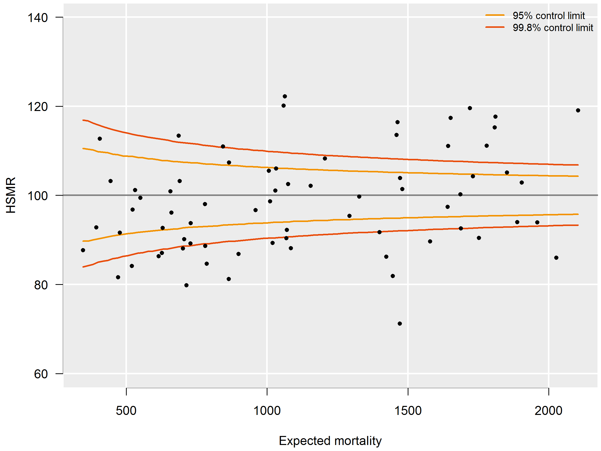
HSMRs can be presented in a funnel plot (see figure 3.6.4): a plot of hospitals, where the vertical axis represents the HSMRs and the horizontal axis the expected mortalities. Hospitals located above the horizontal axis (HSMR=100) have a higher than expected mortality. As this might be a non-significant feature based on chance, control limits are shown in the plot for each possible expected mortality. HSMRs within these control limits do not deviate significantly from 100. In the case of 95 percent control limits, about 2.5 percent of the points would be above the upper limit if there is no reason for differences between HSMRs, and about 2.5 percent of the points below the lower limit. The same holds, mutatis mutandis, for the 99.8 percent control limits. Here about 0.1 percent of the points would be located above the upper line if there is no reason for differences in standardised mortality rates. Most attention will be paid to this line, as points above this line have a high HSMR that is statistically very significant, which can hardly be the result of chance alone. These hospitals would be advised to investigate the possible reasons for the significantly high values: coding errors, unmeasured case mix variables and/or suboptimal quality of care.
The precision of the HSMR is much greater for a three-year period than for a single year, which is reflected by a smaller range between the control limits. The confidence intervals of the HSMR are also smaller. Of course, drawbacks are that two consecutive three-year figures (e.g. 2015-2017 and 2016-2018) overlap, and that the three-year figure is less up-to-date than the figure of the last year. Therefore we also calculated the HSMR figures for the most recent year. Observed mortality (numerator) and expected mortality (denominator) are then calculated for this year’s admissions, whereas the expected mortality model of the HSMR still uses the four-year data. If a hospital has a significantly high HSMR in the most recent year, but not in the three-year period, this is a signal for further investigation, as the quality of care may have deteriorated. There can also be other reasons for this, e.g. differences in registration practices over the years, but it is a signal for the hospital for further investigation.
On the other hand, if a hospital has a significantly high HSMR for the three-year period, but not in the last year, this does not necessarily mean that the situation has improved in the last year, as the one-year figures are less often significant because of the larger margins. In such cases, not only the significance should be taken into account, but also the HSMR levels over the years.
3.6.4 P-Values
From 2017 onwards, it was decided to also calculate p-values for the SMRs of the 158 diagnosis groups. The reason is that high SMRs for diagnosis groups are often an important starting point for further research and hospitals might need an extra tool for prioritizing such research, in case of multiple high SMRs. The lower the p-value, the more likely it is that the observed mortality deviates from the expected mortality. The p-values therefore allow hospitals to investigate their SMRs in order of significance (lowest p-values first). Also, because of the large number of diagnosis groups, there is a risk of incorrectly labelling SMRs as significantly high of low, i.e. the so called type I errors, or false-positives, due to multiple testing (Goeman and Solari, 2011). To reduce this risk, a lower p-value can be chosen as a cut-off. The p-values are not included in the reports sent to the hospitals, but hospitals can request them from Dutch Hospital Data.
Separate p-values are given for the alternative hypotheses: “the observed mortality (Odh) is higher than the expected mortality (Edh)” and “the observed mortality (Odh) is lower than the expected mortality (Edh).” The p-values belonging to the these hypotheses are denoted by Phigh (Odh) and Plow (Odh) respectively. The main reason for calculating two separate p-values is that by using a confidence of 99 percent for each of the two tests results in the same significant SMRs as found with the 98 percent confidence interval of the SMRs. Another reason is that often the main interest is Phigh (Odh).
The p-value of null-hypothesis “the observed mortality is lower or equal to the expected mortality” is given by the probability of observing a mortality equal to or higher than the observed mortality given the expected mortality:
\begin{equation}
p_\mathrm{high}(O_{dh}) = \Pr(X \ge O_{dh} | E_{dh}) = 1 - \Pr(X < O_{dh} | E_{dh})
\end{equation}
Assuming that the observed mortality follows a Poisson-distribution with and expected value equal to the expected mortality this is equal to
\begin{equation}
p_\mathrm{high}(O_{dh}) = 1-P_{E_{dh}}(X \le O_{dh}) + P_{E_{dh}}(X = O_{dh})
\end{equation}
With PEdh(X ≤ Odh) the cumulative distribution function and PEdh(X = Odh) the probability distribution function of the Poisson-distribution with an expected value of Edh.
Likewise the p-value of the null-hypothesis “the observed mortality is higher or equal to the expected mortality” is given by:
\begin{equation}
p_\mathrm{low}(O_{dh}) = P_{E_{dh}}(X \le O_{dh})
\end{equation}
2) For this criterion, all secondary diagnoses are considered, even if they do not belong to the 17 comorbidity groups used as covariates. If identical secondary diagnoses (identical ICD-10 codes) are registered within one admission, only one is counted. If a secondary diagnosis is identical to the main diagnosis of the admission, it is not counted as a secondary diagnosis.