Impact of climate change on economic development
About this publication
We have presented the preliminary findings of two experimental studies in this report. The first study "Impact of anomalous weather conditions on economic sectors" used time series analysis to relate meteorological variables to changes in the value added of various sectors: construction, manufacturing, food & accommodation services, mining & quarrying, and energy. This method allowed us to determine the impact of anomalous weather – and that of climate change – on those sectors over the period 1995 through the second quarter of 2024. The second study ‘Size of the economy in flood-prone areas’, used Geographic Information Systems (GIS) to combine flood risk maps with economic information from the regional accounts from Statistics Netherlands. That information included the value added, production, and employment opportunities. The study showed the scope of these variables in areas with varying levels of flood risk for the period 2010-2022. These studies stem from the societal challenge.
1. Introduction
Climate change is currently one of the biggest challenges for the Dutch economy. Not only do the effects of climate change need to be mitigated – e.g. by limiting greenhouse gas emissions – but we also need to adapt to the effects of climate change. According to projections from the Royal Netherlands Meteorological Institute (KNMI), climate change in the Netherlands will be driven by four different factors (known as pressure factors):
- It will get warmer: both the average temperature and the temperature extremes are going to rise. Heatwaves will increase in frequency, intensity, and duration.
- It will get dryer: the frequency of precipitation will be reduced, which, coupled with an increase in the evaporation of water, will intensify dry spells. It will get wetter: the warmer atmosphere will
- lead to increasing levels of humidity, which will make the few instances of precipitation much more severe.
- Sea levels will rise: sea water temperatures will increase; combined with the melting of the polar ice caps, this will cause sea levels to rise. This will lead to issues such as soil salinisation in coastal areas.
By using the National Climate Adaptation Strategy (NAS) adaptation tool1) we can create conceptual diagrams for different economic sectors, showing the (relevant) consequences of the factors mentioned above. According to the definitions of climate impact and climate risks provided by the IPCC2), the impact of those factors can be subdivided under the terms climate-related hazards, exposure, and vulnerability; the latter term combines sensitivity and adaptive capacity. It is important to monitor all these components in order to design effective mitigation and adaptive policies. Statistical institutes around the world have a part to play in that regard3) .
The research consisted of two parts. The first part, ‘The impact of anomalous weather conditions on economic sectors’, used a time series analysis to relate meteorological variables to changes in the value added of various sectors: construction, manufacturing, food & accommodation services, mining & quarrying, and energy. This method allowed us to determine the impact of anomalous weather – and that of climate change – on those sectors. It can also be used indirectly to determine the factors and climate variables with a significant economic impact. The results of this study are an update of earlier research, which will be explained below in more detail. Additionally, we will provide information on related ongoing research.
The second part of the study, ‘Size of the economy in flood-prone areas’, used Geographic Information Systems (GIS) to combine flood risk maps with economic information from regional accounts from CBS. That information included the value added4) , production, and employment opportunities. The study showed the scope of these variables in areas with varying levels of flood risk.
Summary
Study 1: ‘Impact of anomalous weather conditions on economic sectors’
- We quantified the impact of anomalous weather, using both economic data from CBS and weather data from KNMI of the last three decades.
- The influence of meteorological differences on the economy, such as the numbers of warm days and frost days, is crucial to ascertaining the influence of climate change on the economy; climate change will greatly affect the frequency of these extremes.
- According to the preliminary results, the construction and manufacturing sectors are especially affected by the number of frost days, whereas the food and accommodation services sector is primarily affected by changes in the maximum temperature.
- This study will be refined further and expanded in 2025. Among other changes, we will be adopting a greater selection of weather variables.
Study 2: ‘Size of the economy in flood-prone areas’
- The economy in risk areas can be measured by combining regional economic data from CBS with a map of climate risks.
- For illustrative purposes, this study shows economic figures for several flood risk maps from the National Information System for Water and Floods (LIWO). The figures can be disaggregated by economic sector and by region5).
- One flood scenario concerns the flooding of areas unprotected by the dykes, which repeats once every ten years (‘high risk’ scenario). In that scenario, the flood-prone area encompasses roughly 1 percent of the GDP and Limburg and areas along the Netherlands’ major rivers are especially at risk.
- Another flood scenario involves the breach of primary dams and dykes, which repeats once every 100,000 years (‘extremely low risk’). In this scenario, the flood-prone areas mainly consist of the low-lying areas of the Netherlands and make up around 53 percent of the GDP.
- Additionally, the study shows visible differences between sectors. The energy sector had the largest share of businesses in flood-prone areas, compared to the smallest share for the manufacturing sector
1) https://nas-adaptatietool.nl/, accessed on 11-12-2024.
2) IPCC (Intergovernmental Panel on Climate Change), AR6 Climate Change 2022: Impacts, Adaptation, and Vulnerability. Contribution of working group II to the sixth assessment report, 2022.
3) https://unece.org/statistics/documents/2023/12/informal-documents/guidance-role-national-statistical-offices, accessed on 11-12-2024.
4) The value added equals the production value minus the value of goods and services that are consumed in the production process. The value added of all regional accounts together adds up to the Gross Domestic Product (GDP).
5) Regions were defined using the Coordinating Committee Regional Research Programme (COROP)-plus classification, which distinguishes between 52 different regions.
2. Impact of anomalous weather conditions on economic sectors
2.1 How do we measure the economic impact of anomalous weather?
This part of the study investigated the relationship between climate and the economy through a time series analysis. We were particularly interested in whether anomalies in the weather, compared to normal weather conditions, affected the value added of certain economic sectors, as measured in the CBS national accounts. We used long-series macroeconomic data and weather measurements to estimate those effects. Using an econometric time series model, we reconstructed the structural connections between economic data and weather data. The model described the trends in the economic series, as well as seasonal patterns and possible special series interruptions. It was then enhanced further through the addition of weather variables. These were used to estimate the economic impact of weather anomalies; they also partly explained deviations in the economic trends. The chances of these weather anomalies occurring depend on the climate; as the climate changes, so do those chances. The number of frost days is an example of a weather variable. That number will decrease as a result of climate change, which may affect the output of certain sectors. We aimed to demonstrate that effect in this study by looking at weather and economic data from the past thirty years. By doing so, the study allowed us to show the influence of the (changing) climate in various economic sectors.
An earlier study6) demonstrated which of the tested weather variables has the most statistically significant effect on the following sectors: construction, manufacturing, food & accommodation services, mining & quarrying, and energy, as well as the size of the effect. This chapter’s results are therefore an updated account of prior research. We will discuss plans for refining and expanding said research in section 2.3.
2.2 The effects of weather on the sectors construction, manufacturing, food & accommodation services, mining & quarrying, and energy
2.2.1 Weather variables
We used time series of the weather variables in Table 2.2.1.1.
| Element | Description |
|---|---|
| TG | Daily average temperature (in 0.1°C) |
| TN | Minimum temperature (in 0.1°C) |
| TX | Maximum temperature (in 0.1°C) |
| RH | Daily total precipitation (in 0.1 mm) |
| DR | Daily duration of precipitation (in 0.1 hrs) |
| FG | Daily average wind speed (in 0.1 m/s) |
| FHX | Highest hourly average wind speed (in 0.1 m/s) |
| SQ | Duration of sunshine (in 0.1 hrs) |
| SP | Percentage of the maximum possible duration of sunshine |
Additionally, we created time series for the weather variables in Table 2.2.1.2, based on daily KNMI data.
| Weather variable | Description | |
|---|---|---|
| Frost | If avg. temp. < 0ºC, value = avg. temp. | else value = 0 |
| Dummy frost | If avg. temp. < 0ºC, value = 1 | else value = 0 |
| Deep frost | If avg. temp. < -3ºC, value = avg. temp. | else value = 0 |
| Dummy deep frost | If avg. temp. < -3ºC, value = 1 | else value = 0 |
| Deep frost 7 | If avg. temp. < -7ºC, value = avg. temp. | else value = 0 |
| Dummy deep frost 7 | If avg. temp. < -7ºC, value = 1 | else value = 0 |
| Degree day | If avg. temp. < 18ºC, then value = 18 - avg. temp. | else value = 0 |
| Dummy sunny day | If % sun > 0.5, then value = 1 | else value = 0 |
| Dummy nice day | If % sun > 0.5 AND avg. temp. > 18ºC, then value = 1 | else value = 0 |
| Dummy rainy day | If hours of rain per day > 6, then value = 1 | else value = 0 |
| Dummy snow | If amount of snow in mm. on day t > day t-1, then value = 1 | else value = 0 |
2.2.2 Economic data
Our study used the macro-economic time series from Q1 1995 to Q2 2024. We applied the definition of GDP based on output, as shown in StatLine7) , i.e. based on the value added for each economic sector. Specifically, we selected the following figures for each economic sector:
- value in millions of euros
- measured in constant prices (price level 2021=100)
- not corrected for structural, seasonal fluctuations.
We investigated several sectors of the Standard Industrial Classification (SBI), namely B: Mining and quarrying; C: Manufacturing; D: Energy; F: Construction; and I: Food and accommodation services. We also looked at the sum total of these sectors.
2.2.3 Updating the results
Tables 2.2.3.1 and 2.2.3.2 show the influence of particular weather anomalies in Q4 2023 and Q1 2024. We calculated the effects of the most significant variables for each sector (see Table 2.2.1.2). In the sectors construction and manufacturing, this effect is the result of several days of deep frost; in food and accommodation services, it is the effect of maximum temperatures; and in mining & quarrying, as well as energy, it is the effect of degree days.
| Q4 2023 | Original | Adjusted | Weather effects | y.o.y. (orig., %) | y.o.y. (corr., %) |
|---|---|---|---|---|---|
| Total | 43 445 | 43 312 | 133 | -2.8 | -3.2 |
| Construction | 10 346 | 10 249 | 96 | -1.3 | -2.4 |
| Manufacturing | 25 87 | 25 8 | 70 | -1.6 | -2.0 |
| Food and accommodation services | 4 138 | 4 099 | 38 | -7.1 | -7.1 |
| Mining and Quarrying | 802 | 834 | -33 | -34.9 | -34.2 |
| Energy | 2 289 | 2 327 | -39 | 3.2 | 3.7 |
| 2024-Q1 | Original | Adjusted | Weather effects | y.o.y. (orig., %) | y.o.y. (corr., %) |
|---|---|---|---|---|---|
| Total | 42 473 | 42 307 | 166 | -5.3 | -4.9 |
| Construction | 11 798 | 11 67 | 128 | -5.8 | -4.9 |
| Manufacturing | 23 64 | 23 555 | 85 | -5.6 | -5.2 |
| Food and accommodation services | 3 665 | 3 62 | 45 | 0.5 | 0.0 |
| Mining and Quarrying | 875 | 919 | -44 | -31.0 | -29.8 |
| Energy | 2 495 | 2 542 | -48 | 4.7 | 5.4 |
For each sector, the figure in the column entitled ‘Original’ shows the value added, including the weather effect. ‘Adjusted’ shows what the value added would have been without that weather effect, if weather variables had not deviated from the multi-year average. For example, the adjusted figure for the mining and quarrying sector (919 million) is higher than the actual, original figure (875 million). The true figure is therefore 44 million euros lower than would be expected with average weather conditions. Although there is a clear, observable weather effect in each sector, these effects more or less cancel each other out when looking at the total for all sectors, making it vitally important to conduct further research into smaller aggregates.
Figure 2.2.3.3 to 2.2.3.8 show the magnitude of the weather effect for each sector in all quarters across the full time series. For some sectors (construction and manufacturing), the weather effect is mainly determined by frost. As such, this effect is concentrated in Q1 and Q4, from October to March. In the other sectors, the weather effect is observable throughout the year.
| Jaar | Q1 (million euros) | Q2 (million euros) | Q3 (million euros) | Q4 (million euros) |
|---|---|---|---|---|
| 95 | 36.3 | 127.08 | 2.02 | -117.69 |
| 96 | 304.19 | 249.24 | 133.58 | -100.57 |
| 97 | -535.15 | 132.33 | -15.54 | 155.91 |
| 98 | -155.63 | -36.95 | 47.47 | 279.9 |
| 99 | 30.01 | -30.92 | -76.17 | 174.53 |
| 00 | 116.91 | -34.25 | -3.3 | -33.56 |
| 01 | 329.7 | 67.87 | 32.14 | -100.11 |
| 02 | -64.88 | -32.03 | -31.37 | -58.56 |
| 03 | -56.53 | -70.51 | -0.75 | 347.68 |
| 04 | 337.03 | 2.03 | 0.31 | 196.91 |
| 05 | 159.42 | 35.74 | 3.66 | -17.29 |
| 06 | 686.62 | 7.7 | -59.51 | -229.36 |
| 07 | -54.66 | -167.22 | 30.98 | 86.82 |
| 08 | 175.22 | -70.01 | 36.06 | 128.65 |
| 09 | 284.47 | -79.3 | -48.66 | -129.15 |
| 10 | -143.24 | 155.47 | 36.23 | -245.74 |
| 11 | 295.71 | -168.14 | 23.89 | 14.42 |
| 12 | -889.28 | 72.85 | 29.36 | 161.56 |
| 13 | 105.8 | 252.01 | -3.74 | 0.67 |
| 14 | 25.89 | -126.05 | -39.43 | -93.84 |
| 15 | 384.66 | 82.87 | 33.18 | -95.82 |
| 16 | 206.49 | -24.62 | -74.59 | 119.2 |
| 17 | 127.59 | -38.53 | -6.98 | 69.34 |
| 18 | -12.59 | -122.03 | 13.55 | 105.28 |
| 19 | 228.56 | -1.91 | 0.96 | 130.12 |
| 20 | 253.61 | -44.72 | 8.31 | 94.3 |
| 21 | -210.3 | 59.8 | -42.19 | 38.57 |
| 22 | 356.59 | -4.77 | 31.26 | -65.79 |
| 23 | 383.92 | 13.55 | -6.1 | 132.88 |
| 24 | 165.93 | -20.02 |
| Q1 (million euros) | Q2 (million euros) | Q3 (million euros) | Q4 (million euros) | |
|---|---|---|---|---|
| 95 | 111.12 | 0 | 0 | -297.58 |
| 96 | -852.04 | 0 | 0 | -388.45 |
| 97 | -570.12 | 0 | 0 | 20.49 |
| 98 | 126.60 | 0 | 0 | -70.39 |
| 99 | 111.12 | 0 | 0 | 96.22 |
| 00 | 235.15 | 0 | 0 | 50.78 |
| 01 | 95.64 | 0 | 0 | 20.49 |
| 02 | 188.53 | 0 | 0 | -161.26 |
| 03 | -214.02 | 0 | 0 | 96.22 |
| 04 | 219.84 | 0 | 0 | 65.93 |
| 05 | 80.16 | 0 | 0 | 65.93 |
| 06 | 80.16 | 0 | 0 | 96.22 |
| 07 | 234.98 | 0 | 0 | -9.80 |
| 08 | 250.47 | 0 | 0 | -40.09 |
| 09 | -12.74 | 0 | 0 | -100.68 |
| 10 | -508.19 | 0 | 0 | -494.48 |
| 11 | 157.57 | 0 | 0 | 96.22 |
| 12 | -637.66 | 0 | 0 | 81.08 |
| 13 | -337.88 | 0 | 0 | 96.22 |
| 14 | 234.98 | 0 | 0 | 81.08 |
| 15 | 234.98 | 0 | 0 | 96.22 |
| 16 | 143.28 | 0 | 0 | 35.64 |
| 17 | 95.64 | 0 | 0 | 96.22 |
| 18 | -90.15 | 0 | 0 | 96.22 |
| 19 | 204.02 | 0 | 0 | 96.22 |
| 20 | 250.47 | 0 | 0 | 96.22 |
| 21 | -136.60 | 0 | 0 | 35.64 |
| 22 | 250.47 | 0 | 0 | -24.95 |
| 23 | 250.47 | 0 | 0 | 96.22 |
| 24 | 127.96 | 0 |
| Jaar | Q1 (million euros) | Q2 (million euros) | Q3 (million euros) | Q4 (million euros) |
|---|---|---|---|---|
| 95 | 41.49 | 0 | 0 | -113.35 |
| 96 | -313.96 | 0 | 0 | -152.64 |
| 97 | -210.81 | 0 | 0 | 8.32 |
| 98 | 50.73 | 0 | 0 | -28.97 |
| 99 | 45.01 | 0 | 0 | 43.22 |
| 00 | 102.82 | 0 | 0 | 23.69 |
| 01 | 43.62 | 0 | 0 | 9.55 |
| 02 | 84.32 | 0 | 0 | -74.45 |
| 03 | -95.33 | 0 | 0 | 43.90 |
| 04 | 102.81 | 0 | 0 | 31.18 |
| 05 | 38.26 | 0 | 0 | 32.40 |
| 06 | 39.19 | 0 | 0 | 49.32 |
| 07 | 125.53 | 0 | 0 | -5.26 |
| 08 | 136.02 | 0 | 0 | -20.22 |
| 09 | -5.85 | 0 | 0 | -48.58 |
| 10 | -235.45 | 0 | 0 | -250.58 |
| 11 | 79.50 | 0 | 0 | 49.42 |
| 12 | -322.73 | 0 | 0 | 41.79 |
| 13 | -164.22 | 0 | 0 | 51.27 |
| 14 | 119.06 | 0 | 0 | 43.24 |
| 15 | 119.96 | 0 | 0 | 53.35 |
| 16 | 75.21 | 0 | 0 | 20.26 |
| 17 | 53.70 | 0 | 0 | 58.85 |
| 18 | -53.55 | 0 | 0 | 60.99 |
| 19 | 122.24 | 0 | 0 | 62.58 |
| 20 | 151.22 | 0 | 0 | 63.98 |
| 21 | -88.11 | 0 | 0 | 25.79 |
| 22 | 173.55 | 0 | 0 | -18.43 |
| 23 | 176.09 | 0 | 0 | 69.90 |
| 24 | 84.95 | 0 |
| Jaar | Q1 (million euros) | Q2 (million euros) | Q3 (million euros) | Q4 (million euros) |
|---|---|---|---|---|
| 95 | 5.67 | -29.54 | 26.15 | -18.28 |
| 96 | -80.29 | -32.85 | -36.39 | -38.13 |
| 97 | -18.53 | -29.46 | 16.44 | -11.39 |
| 98 | 27.72 | -4.04 | -45.95 | -45.10 |
| 99 | 7.43 | -4.85 | 32.80 | -3.42 |
| 00 | 11.08 | 13.23 | -37.92 | 5.13 |
| 01 | -26.78 | -25.68 | -12.34 | 18.00 |
| 02 | 34.26 | -2.20 | -4.68 | -21.67 |
| 03 | -3.36 | 29.84 | 40.17 | -14.09 |
| 04 | -3.07 | -5.51 | -2.73 | -7.35 |
| 05 | -8.24 | 6.32 | -15.00 | 20.32 |
| 06 | -54.48 | -3.00 | 58.80 | 59.63 |
| 07 | 51.49 | 49.51 | -41.57 | -14.47 |
| 08 | 21.65 | 19.66 | -24.80 | -26.22 |
| 09 | -31.17 | 21.66 | 12.20 | -3.77 |
| 10 | -49.03 | -19.86 | -10.39 | -57.13 |
| 11 | -1.42 | 40.58 | -32.04 | 24.66 |
| 12 | -3.27 | -24.98 | -12.65 | -4.61 |
| 13 | -58.49 | -43.94 | 6.21 | 18.05 |
| 14 | 43.56 | 14.95 | 4.70 | 26.23 |
| 15 | -3.02 | -19.20 | -7.41 | 52.92 |
| 16 | 1.38 | -5.08 | 30.80 | -7.38 |
| 17 | 7.95 | 27.65 | -16.35 | 16.81 |
| 18 | -22.23 | 65.06 | 53.47 | 31.98 |
| 19 | 29.92 | 22.78 | 22.68 | 11.94 |
| 20 | 30.44 | 12.79 | 20.20 | 8.95 |
| 21 | 0.07 | -19.40 | -8.58 | 11.55 |
| 22 | 33.90 | 25.01 | 47.57 | 40.84 |
| 23 | 27.58 | 26.25 | 24.99 | 38.12 |
| 24 | 44.58 | 20.49 |
| Q1 (million euros) | Q2 (million euros) | Q3 (million euros) | Q4 (million euros) | |
|---|---|---|---|---|
| 95 | -112.88 | 135.77 | -20.24 | 284.25 |
| 96 | 1458.48 | 248.23 | 145.62 | 436.13 |
| 97 | 245.18 | 141.09 | -27.18 | 125.77 |
| 98 | -331.81 | -28.30 | 79.37 | 387.78 |
| 99 | -123.28 | -22.38 | -90.94 | 34.70 |
| 00 | -213.19 | -40.49 | 28.66 | -101.00 |
| 01 | 199.31 | 80.23 | 37.27 | -133.01 |
| 02 | -339.43 | -25.55 | -22.74 | 179.39 |
| 03 | 235.64 | -84.02 | -34.20 | 200.31 |
| 04 | 16.03 | 6.48 | 2.64 | 97.17 |
| 05 | 44.49 | 25.04 | 15.60 | -120.65 |
| 06 | 569.34 | 9.05 | -96.57 | -378.70 |
| 07 | -413.65 | -178.62 | 61.54 | 104.22 |
| 08 | -209.50 | -76.51 | 52.88 | 191.53 |
| 09 | 300.21 | -83.04 | -51.50 | 21.21 |
| 10 | 589.00 | 151.97 | 40.28 | 497.50 |
| 11 | 54.05 | -178.32 | 48.35 | -137.28 |
| 12 | 66.55 | 83.95 | 36.07 | 38.19 |
| 13 | 598.02 | 259.36 | -8.71 | -145.51 |
| 14 | -326.57 | -120.30 | -37.60 | -214.17 |
| 15 | 28.46 | 85.86 | 34.15 | -245.84 |
| 16 | -11.41 | -16.33 | -87.01 | 57.83 |
| 17 | -24.88 | -52.96 | 7.50 | -81.43 |
| 18 | 124.65 | -145.05 | -30.91 | -64.25 |
| 19 | -102.71 | -18.50 | -16.14 | -29.40 |
| 20 | -135.36 | -40.51 | -7.57 | -50.34 |
| 21 | 9.84 | 51.02 | -20.25 | -19.48 |
| 22 | -64.56 | -17.52 | -9.17 | -35.82 |
| 23 | -40.27 | -6.26 | -14.38 | -32.79 |
| 24 | -44.06 | -18.44 |
| Q1 (million euros) | Q2 (million euros) | Q3 (million euros) | Q4 (million euros) | |
|---|---|---|---|---|
| 95 | -9.10 | 20.85 | -3.88 | 27.28 |
| 96 | 92.01 | 33.86 | 24.35 | 42.52 |
| 97 | 19.13 | 20.70 | -4.79 | 12.72 |
| 98 | -28.87 | -4.62 | 14.05 | 36.57 |
| 99 | -10.27 | -3.69 | -18.03 | 3.80 |
| 00 | -18.94 | -6.99 | 5.96 | -12.15 |
| 01 | 17.91 | 13.33 | 7.21 | -15.14 |
| 02 | -32.56 | -4.28 | -3.95 | 19.43 |
| 03 | 20.54 | -16.33 | -6.72 | 21.35 |
| 04 | 1.41 | 1.07 | 0.40 | 9.97 |
| 05 | 4.75 | 4.38 | 3.06 | -15.30 |
| 06 | 52.41 | 1.65 | -21.74 | -55.84 |
| 07 | -53.02 | -38.12 | 11.01 | 12.13 |
| 08 | -23.42 | -13.16 | 7.97 | 23.66 |
| 09 | 34.02 | -17.92 | -9.35 | 2.66 |
| 10 | 60.43 | 23.36 | 6.34 | 58.95 |
| 11 | 6.01 | -30.40 | 7.58 | -18.60 |
| 12 | 7.82 | 13.88 | 5.94 | 5.11 |
| 13 | 68.36 | 36.59 | -1.25 | -19.36 |
| 14 | -45.15 | -20.70 | -6.53 | -30.22 |
| 15 | 4.27 | 16.21 | 6.43 | -52.47 |
| 16 | -1.97 | -3.22 | -18.38 | 12.85 |
| 17 | -4.82 | -13.21 | 1.86 | -21.10 |
| 18 | 28.69 | -42.04 | -9.01 | -19.66 |
| 19 | -24.91 | -6.19 | -5.58 | -11.23 |
| 20 | -43.15 | -17.00 | -4.33 | -24.52 |
| 21 | 4.49 | 28.17 | -13.35 | -14.93 |
| 22 | -36.77 | -12.26 | -7.14 | -27.44 |
| 23 | -29.95 | -6.44 | -16.71 | -38.58 |
| 24 | -47.51 | -22.08 |
2.3 Plans for refining and expanding the study
The figures shown in section 2.2.2 serve as an update to an earlier CBS study on this subject. We hope to refine these results in future research. We will also expand them in terms of the economic data that we wish to explain, the weather effects we wish to investigate, and the econometric time series models we wish to use for that purpose. We have listed the most important suggested improvements for each of these subjects below.
Economic data:
- Our principal focus will be on the agriculture, transportation, and food & accommodation services sectors, as that is where we expect to find clear weather effects. However, we also hope to develop a more general approach that can be applied to other sectors.
- If we look at the economy as a whole, we can also investigate which climate factor – such as drought or extreme precipitation – has the largest effect in which sector.
- In addition to value added per sector, it is also vital that we consider changes in volume and pricing separately. If volumes decrease due to extreme weather conditions (e.g. due to a failed harvest), this could lead to price rises even if turnover (price x volume) remains relatively stable. In other words, certain weather effects will show up in the data of one series, but not in the others.
- In the previous study, we looked at macro-economic quarterly figures. However, some weather effects can be difficult to detect at those frequencies or levels of aggregation because they cancel each other out in sub frequencies and sectors. This is why we plan to look at various levels of aggregation; smaller aggregates could be temporal (e.g. monthly series instead of quarterly) or intrasectional (e.g. several agricultural product sectors within the broader agriculture sector).
Weather data:
- We looked at a limited number of weather effects in the first study, mainly involving temperature (cold and heat). These could only partially explain the economic series, however. In the research that is currently ongoing, we will take a broader set of variables into account, based on multiple data sources, other defined weather variables, and combinations of weather effects. In doing so, we hope to make our research results more compatible with the pressure factors of the KNMI climate scenarios.
Econometric time series models:
- We will look at a larger set of time series models. Finding the best model will be managed through the standard methods of model selection.
- The time series models will take fluctuations into account, such as outliers, fractions, calendar effects, and the disturbances caused by the COVID-19 pandemic. This will ensure that those effects cannot be erroneously attributed to the weather.
- Each sector may be affected by multiple weather variables, so we will look at models with multiple independent variables.
- Because we hope look at a large number of weather effects, we will develop a method for selecting the most influential weather variable per sector.
- The influence of weather effects can vary between quarters. For instance, a warmer winter does not affect the food and accommodation services sector in the same way as a warmer summer does. To account for this, the weather effects will be modelled quarterly.
- Time dependency: we will research whether the influence of a weather effect changes over the years. The construction sector used to be heavily affected by frost, for example, but technical developments may help them to cope with this better.
2.4 Technical explanation
Establishing weather variables
We used the daily data from the KNMI8) to establish weather variables. Data was available for fifty weather stations across the Netherlands, but we only used measurements from the five homogenised stations: De Bilt, De Kooy (Den Helder), Eelde (Groningen), Vlissingen, and Beek (Maastricht). These measurements were then corrected slightly to make time series comparisons easier. Because the five stations are distributed evenly across the Netherlands, the average of their measurements can serve as a proxy for national weather conditions. The measurements were made up of 38 variables, which can be categorised as follows:
- temperature
- precipitation
- sun, clouds
- wind
- air pressure
- vision
- relative humidity
- Calculate the quarterly totals and averages of the variables for each station.
- Calculate the long-term average over those same quarters for each station, and subtract this from step 1. Because we were looking for the influence of weather anomalies, we looked at anomalies in the long-term average.
- Average across all stations
Time series analysis
For our analysis, we used the methodology by Ouwehand and Van Ruth (2014)9), including adaptations presented in Ouwehand (2020)10). Please see those sources for a technical description of time series analyses.
6) https://www.cbs.nl/nl-nl/maatwerk/2020/48/klimaatimpact-op-de-economie, accessed on 18-12-2024.
7) https://opendata.cbs.nl/statline/#/CBS/nl/dataset/85879NED/table?dl=3BED3, accessed on 18-12-2024
8) https://daggegevens.knmi.nl/, accessed on 19-12-2024
9) https://www.cbs.nl/nl-nl/achtergrond/2014/12/how-unusual-weather-influences-gdp, accessed on 18-12-2024
10)https://www.cbs.nl/nl-nl/maatwerk/2020/48/klimaatimpact-op-de-economie, accessed on 18-12-2024.
3. Size of the economy in flood-prone areas
The Netherlands is very vulnerable to flooding. Not only is a major part of the country below sea level, but there are also several large rivers that empty into the sea. That means the risk of flooding comes not just from the sea, but also from elevated river levels, as well as dyke failures11). Climate change increases the risk of extreme amounts of precipitation and leads to rising sea levels, further increasing the risk of flooding. In this part of the study, we quantified the economy of the areas of the Netherlands that are most susceptible to flooding. Specifically, we quantified how much value added and production were generated, and how many employment opportunities , in flood-prone areas with various flood risks.
3.1 How do we measure the size of the economy in flood-prone areas?
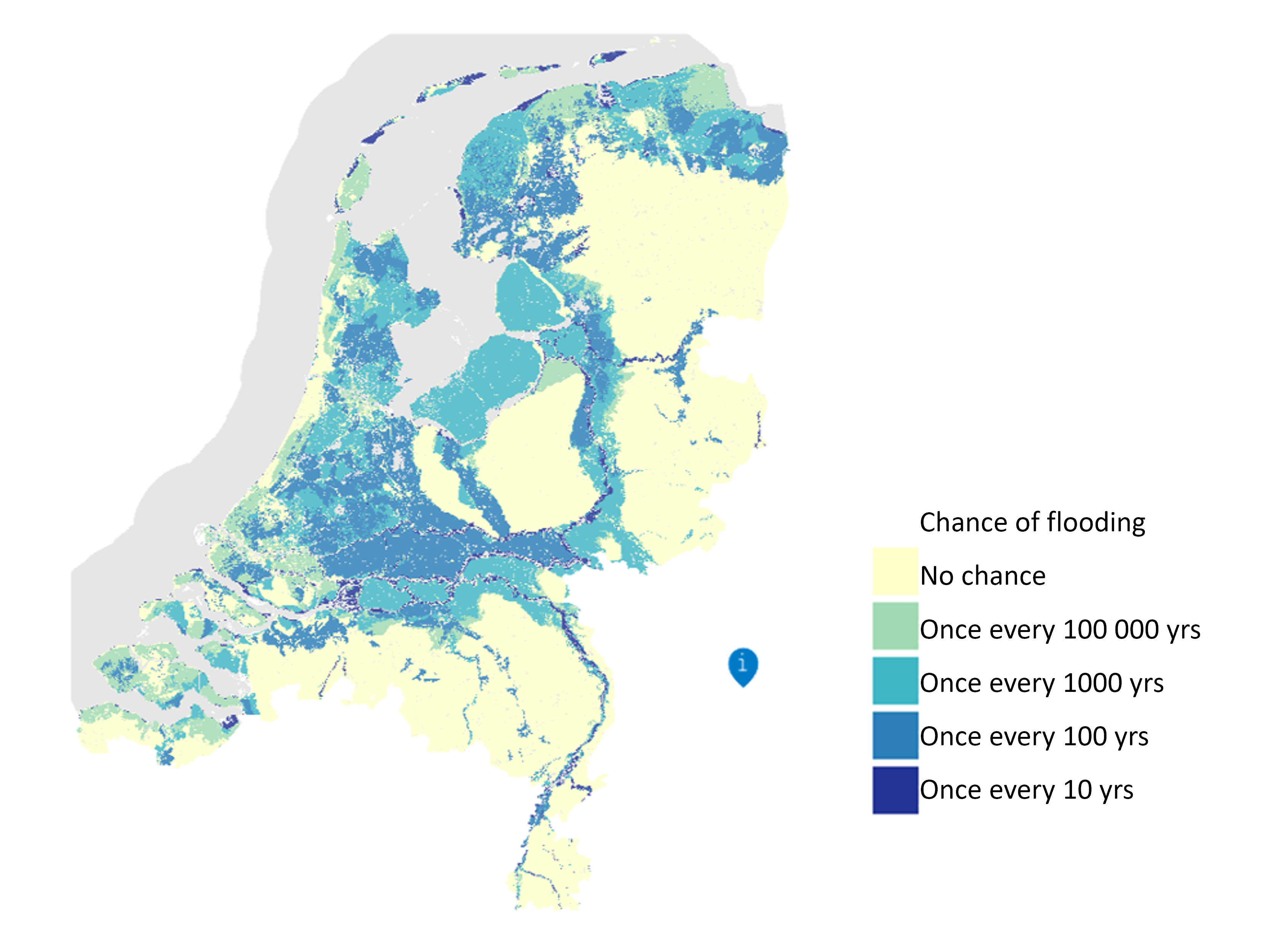
We made use of the LIWO maps of flood-prone areas to quantify the flood risks12). Specifically, we used composites of the water depth maps, which show the maximum depth for certain flood chances, expressed in terms of predicted frequency. The depth was determined based on model simulations. We used three potential flood scenarios identified by the LIWO in our analysis: ‘extremely low risk’ (once every 100 thousand years or less), ‘low risk’ (once every thousand years), and ‘high risk’ (once every 10 years). These maps show potential floods that are unlikely to coincide in reality. They show the combined effect of four types of floods for protected and unprotected areas situated along primary and regional water systems:
A. Flooding of areas close to water, unprotected by dykes
B. Failure of primary dams and dykes
C. Failure of non-primary dams and dykes
D. Flooding from regional water system
We marked all locations where the maximum depth of water is greater than 0 metres as flooded. Several flood scenarios are overlaid in Figure 3.1.1, which shows that, in the ‘high risk’ scenario, floods mainly occur in the areas along the rivers: Limburg, the centre of the Netherlands, and the area around the IJssel river. Flood type A, the flooding of areas unprotected by dykes, is the dominant type in that scenario. The dominant type in the ‘extremely low risk’ scenario is type B, the failure of primary dams and dykes; this is seen on the map as the flooding of Flevoland, Zeeland, Zuid-Holland, and larger areas around the rivers.
Figure 3.1.1 Flood risk map for various scenarios, taken from the Environmental Health Atlas, flooding theme
In order to establish an accurate picture of the economy of flood-prone areas, we linked regional economic data to flood risk maps13) in our analysis. The economic data that we used was sourced from CBS regional accounts, which includes value added, employment opportunities, and production, both per municipality and per economic activity14). For each of these variables, we show what amount is generated in flood-prone areas. However, further analysis is needed to translate that data into information on flood-related economic damage and loss. Such an analysis could also look for correlations between depth and damage, as well as the amount of time that would be needed to repair that damage. While interesting, that analysis is beyond the scope of this study.
Our own analysis provides information on the economy in flood-prone areas for various flood risks. They are grouped according to economic sector and according to region, using the COROP-plus classification15).
3.2 National economy
We will first discuss the economic output generated by flood-prone areas, sorted by flood risk. Gross domestic product (GDP) is generally accepted as a good indicator of economic output, and this is why our analysis looked at the share of the GDP generated in the flood-prone areas shown on the different flood risk maps. As can be seen in Figure 3.2.1, that share was roughly 53 percent in areas with an extremely low risk of flooding. It was 34 percent for areas with a low risk, and a barely 1 percent for high-risk areas. Another point to note is that these percentages have been very stable over the past twenty years16).
However, according to Figure 3.2.2, GDP generated in flood-prone areas is rising sharply in absolute terms. For instance, in the ‘extremely low-risk’ scenario, GDP rose by just under 200 billion euros: from 340 billion euros in 2010 to 525 billion euros in 2022. Given that the chances of flooding are constant, this rise can be explained entirely by the rise in total GDP (see Figure 3.2.1).
| JaarTW | Extremely low risk (for three different levels of flood risk) | Low risk (for three different levels of flood risk) | High risk (for three different levels of flood risk) |
|---|---|---|---|
| 2010 | 53 | 34 | 1 |
| 2012 | 53 | 34 | 1 |
| 2014 | 53 | 34 | 1 |
| 2016 | 53 | 34 | 1 |
| 2018 | 53 | 34 | 1 |
| 2020 | 53 | 34 | 1 |
| 2022 | 53 | 34 | 1 |
| JaarTW | Extremely low risk (Based on three flood risk levels) | Low risk (Based on three flood risk levels) | High risk (Based on three flood risk levels) |
|---|---|---|---|
| 2010 | 339385 | 217934 | 5326 |
| 2012 | 346500 | 222126 | 5416 |
| 2014 | 358016 | 230844 | 5569 |
| 2016 | 381169 | 245879 | 5950 |
| 2018 | 416034 | 268645 | 6520 |
| 2020 | 431024 | 278268 | 6909 |
| 2022 | 524950 | 338032 | 8133 |
3.3 Differences between sectors
Our analysis of GDP can be supplemented by looking at the different economic sectors. We used economic data from 2022 for the following analysis.
Table 3.3.1 shows the impact of the ‘extremely low risk’ scenario on various sectors. We calculated the full-time equivalents (FTEs), value added, and production for each flood-prone area.
Value added generated in flood-prone area
Figure 3.3.2 shows the amount of value added generated in different sectors in areas likely to flood in the ‘extremely low risk’ scenario. As can be seen, in the ‘extremely low risk’ scenario the energy sector had the largest percentage of value added: almost 70 percent was generated in flood-prone areas. That percentage was around 50 percent for most other sectors, down to as low as 42 percent for the manufacturing sector. This is probably because much of the economic activity in that sector (15 percent of value added) is localised around Eindhoven17), where little to no flooding occurs. This compensated for areas like the Rijnmond region (around Rotterdam), which contains 7 percent of the Dutch manufacturing sector and 85 percent of which would flood in the ‘extremely low risk’ scenario.
Figure 3.3.3 shows the absolute GDP values generated in areas at risk of flooding. The values are grouped by sector and by risk scenario. The sector ‘Trade, transport, hotels, catering’ had the largest absolute GDP value: 102 billion, 69 billion, and 2 billion euros for the three different risk scenarios. The public sector and health care come in second place. In terms of value added, these sectors are also the largest at the national level.
The largest share of value added in the energy sector comes from the Rijnmond and Groningen areas (including Eemshaven)18). In each of those areas, more than 80 percent is likely to flood in the ‘extremely low risk’ scenario. The energy sector is also the only sector in which an increasingly large share of value added is generated in flood-prone areas, whereas that variable barely changes in the other sectors. For the energy sector, the share increased from 60 to almost 70 percent between 2010 and 2022 (in the ‘extremely low risk’ scenario). This is mainly due to growth in this sector in regions where flooding occurs over large areas, specifically the regions surrounding Amsterdam19), Flevoland, Rijnmond, and Groningen (including Eemshaven).
Employment in risk areas
We performed a similar analysis on employment figures, as expressed in FTEs. Like the earlier analysis, this one shows which sectors are relatively sensitive to flood risks and which sectors generate the most jobs in risk areas.
As was the case for value added, the energy sector is the most sensitive sector in terms of employment, along with the information and communication sector. In the ‘extremely low risk’ scenario, almost 60 percent of the employment opportunities in those sectors were generated in flood-prone areas. Over 33 percent of employment in the information sector came from the Amsterdam and Utrecht areas, of which 64 and 72 percent would be flooded, respectively, in this scenario. This means that 40 percent of total employment in risk areas can be attributed to these two regions. However, the differences in percentages are much smaller for employment than they are for value added. In almost all sectors in this scenario, between 50 and 60 percent of employment was generated in flood-prone areas, the only exception being manufacturing at 43 percent. The two regions with the most employment in this sector (Eindhoven and Twente, 11 and 5 percent of the national total, respectively) hardly ever flood.
For all three scenarios, public sector and health care had the largest absolute number of jobs in risk areas; it was also the largest sector in terms of jobs in general.
| Employment | Value added | Production | |||||||
|---|---|---|---|---|---|---|---|---|---|
| Flood-prone area | Netherlands total | Percent share | Flood-prone area | Netherlands total | Percent share | Flood-prone area | Netherlands total | Percent share | |
| Economic sector | x 1 000 FTEs | % | mln euros | mln euros | % | mln euros | mln euros | % | |
| Agriculture, forestry and fishing | 46 | 85 | 54 | 7 814 | 16 318 | 48 | 21 224 | 45 171 | 47 |
| Mining and quarrying | 4 | 7 | 51 | 5 933 | 9 254 | 64 | 8 217 | 13 252 | 62 |
| Manufacturing | 272 | 640 | 43 | 43 682 | 102 836 | 42 | 218 2 | 469 319 | 46 |
| Energy | 17 | 29 | 58 | 10 89 | 15 788 | 69 | 23 679 | 34 693 | 68 |
| Water and waste management | 18 | 35 | 52 | 2 764 | 5 166 | 54 | 7 645 | 14 526 | 53 |
| Construction | 168 | 321 | 52 | 23 318 | 43 981 | 53 | 79 913 | 149 842 | 53 |
| Trade, transport, hotels, catering | 847 | 1 582 | 54 | 102 119 | 181 768 | 56 | 212 653 | 375 055 | 57 |
| Information and communication | 167 | 290 | 58 | 26 003 | 44 323 | 59 | 58 625 | 100 459 | 58 |
| Financial services | 105 | 190 | 55 | 29 588 | 51 766 | 57 | 52 719 | 93 821 | 56 |
| Renting buying and selling of real estate | 32 | 60 | 54 | 32 004 | 61 45 | 52 | 53 492 | 102 655 | 52 |
| Business services | 687 | 1 279 | 54 | 81 379 | 145 331 | 56 | 162 496 | 286 252 | 57 |
| Public sector and health care | 1 017 | 2 026 | 50 | 92 914 | 181 592 | 51 | 139 91 | 272 807 | 51 |
| Culture, recreation and other services | 106 | 201 | 53 | 10 739 | 20 027 | 54 | 22 091 | 41 163 | 54 |
| Total macro economy | 3 486 | 6 742 | 52 | 469 146 | 879 6 | 53 | 1 060 866 | 1 999 015 | 53 |
| Macroeconomic total | 524 927 | 984 184 | 53 | ||||||
| Approximate GDP | |||||||||
| A10_Omschrijving | Extremely low risk | Low risk | High risk |
|---|---|---|---|
| Agriculture, forestry and fishing | 48 | 32 | 1 |
| Mining and quarrying | 64 | 39 | 0 |
| Manufacturing | 42 | 29 | 1 |
| Energy supply | 69 | 42 | 2 |
| Water supply and waste management | 54 | 36 | 1 |
| Construction | 53 | 37 | 1 |
| Trade, transport, hotels, catering | 56 | 38 | 1 |
| Information and communications | 59 | 38 | 0 |
| Financial services | 57 | 34 | 0 |
| Real estate activities | 52 | 33 | 1 |
| Business services | 56 | 35 | 1 |
| Public sector and health care | 51 | 31 | 1 |
| Culture, recreation and other services | 54 | 33 | 1 |
| A10_Omschrijving | Extremely low risk | Low risk | High risk |
|---|---|---|---|
| Agriculture, forestry and fishing | 7814 | 5173 | 161 |
| Mining and quarrying | 5933 | 3602 | 44 |
| Manufacturing | 43682 | 30287 | 1119 |
| Energy supply | 10890 | 6630 | 318 |
| Water supply and waste management | 2764 | 1841 | 58 |
| Construction | 23318 | 16482 | 341 |
| Trade, transport, hotels, catering | 102119 | 68726 | 1732 |
| Information en communication | 26003 | 17029 | 183 |
| Financial services | 29588 | 17788 | 150 |
| Real estate activities | 32004 | 20564 | 474 |
| Business services | 81379 | 51169 | 986 |
| Public sector, health care | 92914 | 56281 | 1556 |
| Culture, recreation and other services | 10739 | 6526 | 146 |
3.4 Highest-risk areas in the Netherlands
The method that we chose to measure the economy of flood-prone areas made it possible to analyse various economic sectors, and also to look at the economy of each individual region.
Figure 3.4.1 and Figure 3.4.2 show the variation in the value added in the different risk areas in the ‘extremely low risk’ scenario. The provinces of Flevoland and Zuid-Holland stand out in particular when looking at the at-risk percentage of value added per region. That area is largest in the Betuwe-20) and Delfzijl regions, where respectively 96 and 95 percent of value added is generated in areas with a significant flood risk.
The Rotterdam (Rijnmond) and Amsterdam regions have the highest at-risk value added in absolute terms. These regions generate roughly 61 billion euros in value added in flood-prone areas in the ‘extremely low risk’ scenario.
| Corop_plus_naam | Percentage share of value added ( %) |
|---|---|
| Achterhoek | 36 |
| Aggl. 's-Gravenhage excl. Zoetermeer | 75 |
| Agglomeratie Haarlem | 7 |
| Agglomeratie Leiden en Bollenstreek | 65 |
| Alkmaar en omgeving | 59 |
| Almere | 95 |
| Amsterdam | 64 |
| Arnhem/Nijmegen | 61 |
| Delft en Westland | 68 |
| Delfzijl en omgeving | 95 |
| Drechtsteden | 85 |
| Edam-Volendam en omgeving | 79 |
| Flevoland-Midden | 89 |
| Haarlemmermeer en omgeving | 85 |
| Het Gooi en Vechtstreek | 24 |
| IJmond | 30 |
| Kop van Noord-Holland | 80 |
| Midden-Limburg | 17 |
| Midden-Noord-Brabant | 22 |
| Noord-Drenthe | 2 |
| Noord-Friesland | 46 |
| Noord-Limburg | 22 |
| Noord-Overijssel | 75 |
| Noordoostpolder en Urk | 85 |
| Oost-Groningen | 36 |
| Oost-Zuid-Holland | 90 |
| Overig Agglomeratie Amsterdam | 91 |
| Overig Groningen | 55 |
| Overig Groot-Rijnmond | 71 |
| Overig Noordoost-Noord-Brabant | 26 |
| Overig Zeeland | 79 |
| Overig Zuidoost-Zuid-Holland | 94 |
| Rijnmond | 85 |
| Stadsgewest 's-Hertogenbosch | 88 |
| Stadsgewest Amersfoort | 56 |
| Stadsgewest Utrecht | 67 |
| Twente | 4 |
| Utrecht-West | 85 |
| Veluwe | 17 |
| West-Noord-Brabant | 14 |
| Zaanstreek | 76 |
| Zeeuwsch-Vlaanderen | 31 |
| Zoetermeer | 95 |
| Zuid-Limburg | 13 |
| Zuidoost-Drenthe | 4 |
| Zuidoost-Friesland | 6 |
| Zuidoost-Noord-Brabant | 4 |
| Zuidoost-Utrecht | 63 |
| Zuidwest-Drenthe | 5 |
| Zuidwest-Friesland | 63 |
| Zuidwest-Gelderland | 96 |
| Zuidwest-Overijssel | 59 |
| Totale macro economie | 53 |
| Corop_plus_naam | Value added of flood-prone area ( million euros) |
|---|---|
| Achterhoek | 5165 |
| Aggl. 's-Gravenhage excl. Zoetermeer | 28056 |
| Agglomeratie Haarlem | 570 |
| Agglomeratie Leiden en Bollenstreek | 11483 |
| Alkmaar en omgeving | 5268 |
| Almere | 7281 |
| Amsterdam | 61050 |
| Arnhem/Nijmegen | 20172 |
| Delft en Westland | 8790 |
| Delfzijl en omgeving | 2522 |
| Drechtsteden | 10124 |
| Edam-Volendam en omgeving | 3141 |
| Flevoland-Midden | 5425 |
| Haarlemmermeer en omgeving | 21854 |
| Het Gooi en Vechtstreek | 2797 |
| IJmond | 2181 |
| Kop van Noord-Holland | 10176 |
| Midden-Limburg | 1544 |
| Midden-Noord-Brabant | 4648 |
| Noord-Drenthe | 118 |
| Noord-Friesland | 5762 |
| Noord-Limburg | 2913 |
| Noord-Overijssel | 13274 |
| Noordoostpolder en Urk | 2499 |
| Oost-Groningen | 1904 |
| Oost-Zuid-Holland | 10769 |
| Overig Agglomeratie Amsterdam | 10312 |
| Overig Groningen | 12709 |
| Overig Groot-Rijnmond | 4781 |
| Overig Noordoost-Noord-Brabant | 4545 |
| Overig Zeeland | 9019 |
| Overig Zuidoost-Zuid-Holland | 5272 |
| Rijnmond | 61088 |
| Stadsgewest 's-Hertogenbosch | 14137 |
| Stadsgewest Amersfoort | 8421 |
| Stadsgewest Utrecht | 37156 |
| Twente | 1037 |
| Utrecht-West | 4484 |
| Veluwe | 5211 |
| West-Noord-Brabant | 4119 |
| Zaanstreek | 4269 |
| Zeeuwsch-Vlaanderen | 1396 |
| Zoetermeer | 5055 |
| Zuid-Limburg | 3173 |
| Zuidoost-Drenthe | 213 |
| Zuidoost-Friesland | 483 |
| Zuidoost-Noord-Brabant | 1825 |
| Zuidoost-Utrecht | 4021 |
| Zuidwest-Drenthe | 261 |
| Zuidwest-Friesland | 2978 |
| Zuidwest-Gelderland | 10055 |
| Zuidwest-Overijssel | 3638 |
| Totale macro economie | 469146 |
| Corop_plus_naam | Value added percentage share ( %) |
|---|---|
| Achterhoek | 0 |
| Aggl. 's-Gravenhage excl. Zoetermeer | 1 |
| Agglomeratie Haarlem | 0 |
| Agglomeratie Leiden en Bollenstreek | 0 |
| Alkmaar en omgeving | 0 |
| Almere | 0 |
| Amsterdam | 0 |
| Arnhem/Nijmegen | 0 |
| Delft en Westland | 0 |
| Delfzijl en omgeving | 0 |
| Drechtsteden | 3 |
| Edam-Volendam en omgeving | 2 |
| Flevoland-Midden | 0 |
| Haarlemmermeer en omgeving | 0 |
| Het Gooi en Vechtstreek | 0 |
| IJmond | 0 |
| Kop van Noord-Holland | 0 |
| Midden-Limburg | 12 |
| Midden-Noord-Brabant | 0 |
| Noord-Drenthe | 0 |
| Noord-Friesland | 1 |
| Noord-Limburg | 17 |
| Noord-Overijssel | 1 |
| Noordoostpolder en Urk | 0 |
| Oost-Groningen | 0 |
| Oost-Zuid-Holland | 1 |
| Overig Agglomeratie Amsterdam | 0 |
| Overig Groningen | 0 |
| Overig Groot-Rijnmond | 1 |
| Overig Noordoost-Noord-Brabant | 1 |
| Overig Zeeland | 0 |
| Overig Zuidoost-Zuid-Holland | 1 |
| Rijnmond | 1 |
| Stadsgewest 's-Hertogenbosch | 0 |
| Stadsgewest Amersfoort | 0 |
| Stadsgewest Utrecht | 0 |
| Twente | 0 |
| Utrecht-West | 0 |
| Veluwe | 0 |
| West-Noord-Brabant | 0 |
| Zaanstreek | 0 |
| Zeeuwsch-Vlaanderen | 0 |
| Zoetermeer | 0 |
| Zuid-Limburg | 4 |
| Zuidoost-Drenthe | 0 |
| Zuidoost-Friesland | 0 |
| Zuidoost-Noord-Brabant | 0 |
| Zuidoost-Utrecht | 0 |
| Zuidwest-Drenthe | 0 |
| Zuidwest-Friesland | 5 |
| Zuidwest-Gelderland | 2 |
| Zuidwest-Overijssel | 0 |
| Totale macro economie | 1 |
| Corop_plus_naam | Value added generated in flood-prone area ( million euros) |
|---|---|
| Achterhoek | 2 |
| Aggl. 's-Gravenhage excl. Zoetermeer | 217 |
| Agglomeratie Haarlem | 0 |
| Agglomeratie Leiden en Bollenstreek | 1 |
| Alkmaar en omgeving | 0 |
| Almere | 0 |
| Amsterdam | 2 |
| Arnhem/Nijmegen | 62 |
| Delft en Westland | 0 |
| Delfzijl en omgeving | 13 |
| Drechtsteden | 351 |
| Edam-Volendam en omgeving | 63 |
| Flevoland-Midden | 10 |
| Haarlemmermeer en omgeving | 0 |
| Het Gooi en Vechtstreek | 3 |
| IJmond | 6 |
| Kop van Noord-Holland | 44 |
| Midden-Limburg | 1160 |
| Midden-Noord-Brabant | 57 |
| Noord-Drenthe | 5 |
| Noord-Friesland | 136 |
| Noord-Limburg | 2197 |
| Noord-Overijssel | 150 |
| Noordoostpolder en Urk | 2 |
| Oost-Groningen | 0 |
| Oost-Zuid-Holland | 80 |
| Overig Agglomeratie Amsterdam | 0 |
| Overig Groningen | 93 |
| Overig Groot-Rijnmond | 53 |
| Overig Noordoost-Noord-Brabant | 215 |
| Overig Zeeland | 45 |
| Overig Zuidoost-Zuid-Holland | 39 |
| Rijnmond | 478 |
| Stadsgewest 's-Hertogenbosch | 18 |
| Stadsgewest Amersfoort | 27 |
| Stadsgewest Utrecht | 13 |
| Twente | 5 |
| Utrecht-West | 8 |
| Veluwe | 48 |
| West-Noord-Brabant | 72 |
| Zaanstreek | 0 |
| Zeeuwsch-Vlaanderen | 6 |
| Zoetermeer | 0 |
| Zuid-Limburg | 1055 |
| Zuidoost-Drenthe | 0 |
| Zuidoost-Friesland | 26 |
| Zuidoost-Noord-Brabant | 7 |
| Zuidoost-Utrecht | 1 |
| Zuidwest-Drenthe | 0 |
| Zuidwest-Friesland | 242 |
| Zuidwest-Gelderland | 248 |
| Zuidwest-Overijssel | 6 |
| Totale macro economie | 7268 |
We also looked at the value added in the ‘high risk’ scenario; see Figure 3.4.3 and Figure 3.4.4. The major flood-prone areas in this scenario are Limburg and the areas along the major rivers. Consequently, that is where the economic risks are greatest. Of the value added in North Limburg, 17 percent (2 billion euros) is generated in at-risk areas.
3.5 Major differences by sector and region
In addition to differences between regions and sectors, we can also look at the effect on sectors by region.21)
This report shows the results for the following three COROP-plus regions: Utrecht City, Southeast Utrecht, Southwest Gelderland (see Figure 3.5.1). These regions were selected because, despite bordering each other, they demonstrate major differences in the (relative and absolute) amounts of value added generated in at-risk areas.
| Corop_plus_naam | Value added, percentage share ( %) |
|---|---|
| Achterhoek | 0 |
| Aggl. 's-Gravenhage excl. Zoetermeer | 0 |
| Agglomeratie Haarlem | 0 |
| Agglomeratie Leiden en Bollenstreek | 0 |
| Alkmaar en omgeving | 0 |
| Almere | 0 |
| Amsterdam | 0 |
| Arnhem/Nijmegen | 0 |
| Delft en Westland | 0 |
| Delfzijl en omgeving | 0 |
| Drechtsteden | 0 |
| Edam-Volendam en omgeving | 0 |
| Flevoland-Midden | 0 |
| Haarlemmermeer en omgeving | 0 |
| Het Gooi en Vechtstreek | 0 |
| IJmond | 0 |
| Kop van Noord-Holland | 0 |
| Midden-Limburg | 0 |
| Midden-Noord-Brabant | 0 |
| Noord-Drenthe | 0 |
| Noord-Friesland | 0 |
| Noord-Limburg | 0 |
| Noord-Overijssel | 0 |
| Noordoostpolder en Urk | 0 |
| Oost-Groningen | 0 |
| Oost-Zuid-Holland | 0 |
| Overig Agglomeratie Amsterdam | 0 |
| Overig Groningen | 0 |
| Overig Groot-Rijnmond | 0 |
| Overig Noordoost-Noord-Brabant | 0 |
| Overig Zeeland | 0 |
| Overig Zuidoost-Zuid-Holland | 0 |
| Rijnmond | 0 |
| Stadsgewest 's-Hertogenbosch | 0 |
| Stadsgewest Amersfoort | 0 |
| Stadsgewest Utrecht | 10 |
| Twente | 0 |
| Utrecht-West | 0 |
| Veluwe | 0 |
| West-Noord-Brabant | 0 |
| Zaanstreek | 0 |
| Zeeuwsch-Vlaanderen | 0 |
| Zoetermeer | 0 |
| Zuid-Limburg | 0 |
| Zuidoost-Drenthe | 0 |
| Zuidoost-Friesland | 0 |
| Zuidoost-Noord-Brabant | 0 |
| Zuidoost-Utrecht | 10 |
| Zuidwest-Drenthe | 0 |
| Zuidwest-Friesland | 0 |
| Zuidwest-Gelderland | 10 |
| Zuidwest-Overijssel | 0 |
| Totale macro economie | 0 |
| A10_Omschrijving | Stadsgewest Utrecht | Zuidoost-Utrecht | Zuidwest-Gelderland |
|---|---|---|---|
| Agriculture, forestry and fishing | 81 | 49 | 96 |
| Mining and quarrying | 70 | 12 | 96 |
| Manufacturing | 68 | 88 | 96 |
| Energy supply | |||
| Water supply and waste management | |||
| Construction | 76 | 73 | 96 |
| Trade, transport, hotels, catering | 72 | 79 | 96 |
| Information and communication | 73 | 82 | 96 |
| Financial services | 63 | 26 | 96 |
| Real estate activities | 66 | 59 | 96 |
| Business services | 69 | 65 | 96 |
| Public sector and health care | 63 | 41 | 96 |
| Culture, recreation and other services | 64 | 55 | 96 |
Figure 3.5.2: Percentage of value added in flood-prone areas for three COROP-plus regions, by sector, ‘Extremely low risk’ scenario, economic data from 2022. Data on the energy and the water supply & waste management sectors cannot be shown for reasons of confidentiality.
| A10_Omschrijving | Stadsgewest Utrecht | Zuidoost-Utrecht | Zuidwest-Gelderland |
|---|---|---|---|
| Agriculture, forestry and fishing | 127 | 40 | 548 |
| Mining and quarrying | 20 | 0 | 21 |
| Manufacturing | 1621 | 550 | 1271 |
| Energy supply | |||
| Water supply and waste management | |||
| Construction | 1867 | 261 | 793 |
| Trade, transport, hotels, catering | 6471 | 1036 | 2965 |
| Information and communication | 3767 | 465 | 270 |
| Financial services | 4759 | 114 | 138 |
| Real estate activities | 2121 | 343 | 740 |
| Business services | 6365 | 567 | 1608 |
| Public sector and health care | 8522 | 568 | 1438 |
| Culture, recreation and other services | 1078 | 72 | 161 |
Figure 3.5.3: Share of value added in flood-prone areas for three COROP-plus regions, by sector. ‘Extremely low risk’ scenario, economic data from 2022. Data on the energy and water supply & waste management sectors cannot be shown in this breakdown by region.
Figure 3.5.2 clearly shows major differences between these three adjoining COROP-plus regions. In Southwest Gelderland (the Betuwe region), 96 percent of the value added for all sectors is generated in flood-prone areas. The percentage varies from 60 to 80 percent in Utrecht City, depending on the sector. For most sectors, the smallest share of at-risk value added is generated in the Southeast Utrecht region: between 12 and 88 percent.
The area of Utrecht City that is at risk of flooding is smaller than that of Southwest Gelderland, in relative terms. Nevertheless, Figure 3.5.5 clearly shows that Utrecht City has the highest absolute value added for flood-prone areas across all sectors. Public sector and health care and the trade, transport, and food & accommodation services sector have the largest absolute value added in flood-prone areas. The same is true at the national level (see Figure 3.3.3). In Utrecht City, the public sector and health care are the most at-risk, whereas at the national level this is the case for the trade sector.
3.6 Summary and further research
In this study, we have linked maps showing climate risks with economic data. More specifically, we have combined flood risk maps with several different economic variables. The approach adopted could also be used to investigate other climate threats, coupled with a wider range of economic variables.
In this report, we measured the economy of flood-prone areas in the Netherlands. Among other things, the report shows to what extent value added is generated in areas at risk of flooding, as well as the absolute value added. Using our chosen methodology, we were able to investigate the variables stated, both by sector and by region. Our use of economic activity figures (i.e. value added, production, and employment) at a regional level complements earlier research on flood damage done by Deltares22) and De Nederlandsche Bank (DNB)23). DNB analysed the amount of damage incurred by companies to fixed assets due to flooding. Meanwhile, Deltares’ Damage and Fatality assessment model used the national accounts of Statistics Netherlands (CBS) to calculate the damages caused by business interruptions. For this study, we analysed several different possible flooding scenarios.
We found that, under the ‘extremely low risk’ scenario, roughly 53 percent of the Netherlands’ GDP came from flood-prone areas. This was only 1 percent under the ‘high risk’ scenario. Additionally, the percentages were found to have been stable over the past twenty years. However, GDP value in the flood zones did rise from 340 billion euros to 525 billion euros between 2010 and 2022. This can be explained by the period of GDP growth that started in 2010.
There were also major differences between the economic sectors in terms of the share of value added in flood-prone areas. That share was nearly 70 percent for the energy sector under the ‘extremely low risk’ scenario, compared to slightly over 40 percent for the manufacturing sector.
The different scenarios greatly affected regions’ vulnerabilities relative to each other. Under the ‘extremely low risk’ scenario, the Betuwe and Delfzijl regions were the most vulnerable of all regions: 95 percent of their value added came from areas at risk of flooding. The value added in at-risk areas in the Rijnmond and Amsterdam regions amounted to 61 billion euros per region, making them the highest in absolute terms. Limburg was especially vulnerable under the ‘high risk’ scenario, both in relative and absolute terms: 17 percent of North Limburg’s value added, roughly 2 billion euros, came from at-risk areas.
Possibilities for further research
The notion of linking regional economic data to climate risk maps offers many opportunities. For instance, it can be used to show the Netherlands’ vulnerability to climate risks. To demonstrate this, we investigated which amounts of value added, employment, and production came from areas at risk of flooding. This analysis could be further expanded upon in several ways.
The use of flood data means that there are many maps available for analysis. While our study used the aggregated risk of four different flood scenarios, future research might focus on one specific scenario, such as ‘Flooding of areas next to water, unprotected by dykes’. Another possibility would involve looking at the (combinations of) local flood risk scenarios available from the LIWO. We published economic data at the COROP-plus level for the current study, but these regions are too large to show the economic effects of more localised flooding. Unfortunately, it will take considerable work to find out which municipalities have enough economic data available to be able to carry out research at that level.
A final possibility involves using our analysis for other climate threats like drought, extreme precipitation, and heat. However, this would require investigating how to demarcate the risk areas for each of those threats. And, as with the potential study on local scenarios, it would first be necessary to ascertain whether there is enough economic data available for study (and publication) at the right level of aggregation.
3.7 Technical explanation
Flood maps
As explained in section 3.1, this research used flood maps from the National Information System Water and Floods (LIWO). These maps show the risk of various kinds of flooding in the Netherlands; the map resolution is 25 by 25 metres. More specifically, we used the map entitled Maximum depth of flooding in the Netherlands (‘Maximale overstromingsdiepte Nederland’). This map shows the maximum water depth across the Netherlands for various flood risks. There are five different versions of the map: 1) extremely low risk, 2) very low risk, 3) low risk, 4) medium risk, and 5) high risk. Our analyses focused on maps 1, 3, and 5.
- 1) Extremely low risk: shows which areas should flood once every 100 thousand years (or less).
- 3) Low risk: shows which areas should flood once every thousand years.
- 5) High risk: shows which areas should flood once every 10 years.
All these maps show flooding that in reality would be unlikely to occur simultaneously. The maps are based on four types of flooding of protected and unprotected areas, situated along primary and regional water systems.
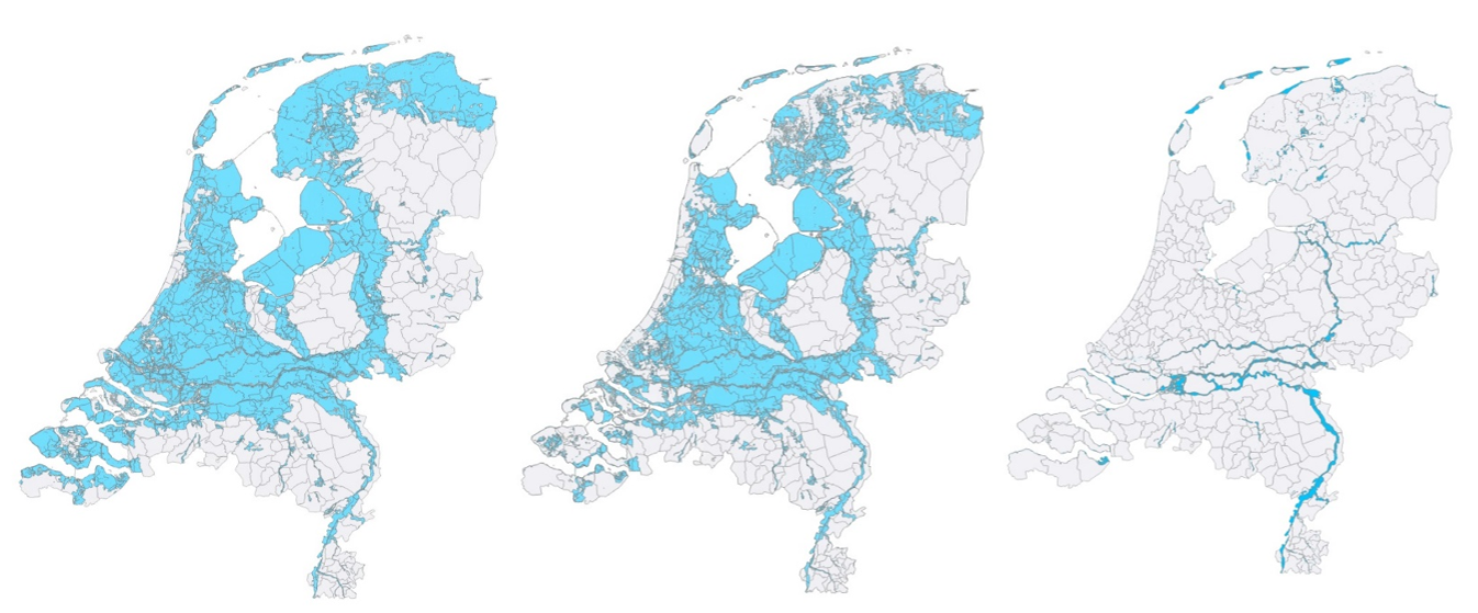
Before performing our analysis, we first discretised the flood map. Every location where depth of water was greater than 0 metres was marked as flooded, which provided us with the maps shown in Figure 3.7.1. These maps therefore no longer differentiate between various depths.
Determining the flooding percentage for each municipality
For each municipality, we determined how much would be subject to flooding. This was not done using the flooded surface area for a given municipality24), but rather using the number of businesses flooded in a municipality. The GIS analysis was done using data from the Basic Register of Addresses and Buildings (BAG). As part of the analysis, every building with the status ‘Object in use’ (Verblijfsobject in gebruik) and any function other than ‘residential’ (woonobject) was counted as a business. This is how we calculated the percentage of businesses flooded in each municipality; this was a much more suitable method for linking economic activities to flood maps than using the surface areas flooded.
Figure 3.7.1 Flood maps after discretisation. From left to right: 1) extremely low risk, 3) low risk, 5) high risk. The lines on the map represent municipal boundaries
Economic data
The economic data we used was sourced from the CBS regional accounts. Those accounts contain economic information broken down by year, municipality, and REGKOL level; it includes figures on value added, production, and employment, among others. Where necessary, the figures for specific companies were broken down by municipality, based on the number of jobs in each municipality. The REGKOL classification is based on the SBI, but on a lower level of aggregation than the national accounts classification, which is itself based on the SBI. Regional accounts are published at the COROP-plus level, aggregated to 21 economic sectors. We opted to use the same level of aggregation for this publication.
The economic data also contains data on extraterritorial regions, whose economic activities cannot be ascribed to a particular region or municipality within Dutch borders. Those activities include work in Dutch embassies abroad, military missions, or mining and quarrying on the Dutch part of the continental shelf. This data was not included in this study.
Linking flood maps to economic data
Linking the maps of flooded areas to economic data was an important step in analysing the data from those areas. Both the maps and the data are available at the municipal level, and were linked at that same level. The percentage of flooded business per municipality was applied to all economic variables. All the time series in this analysis used the same flood risk maps, combined with economic data from the relevant year.
11) Flooding | Environmental Health Atlas, accessed on 10-01-2025.
12) https://basisinformatie-overstromingen.nl/#/maps, accessed on 10-01-2025.
13) The methodology used to link them will be explained in section 3.7.
14) These activities are at REGKOL level; see section 3.7 for more information.
15) For more information on COROP-plus, go to: Landelijk dekkende indelingen | CBS (Dutch only); for an interactive map of COROP-plus regions, go to: 3. Groei per regio | CBS (Dutch only).
16) This analysis was based on the same flood risk maps every year, but we did vary the economic data used; we operated under the assumption that economic changes were much greater than changes in flood risks due to newly constructed or improved dykes.
17) COROP-plus region: Southeast Noord-Brabant
18) COROP-plus region: Remainder Groningen
19) COROP-plus region: Remaining sprawl Amsterdam
20) COROP-plus area Southwest Gelderland
21) For reasons of confidentiality, the data for the energy- and the water supply & waste management sectors cannot be shown at the COROP level.
22) Deltares, Standaardmethode 2017 Schade en slachtoffers als gevolg van overstromingen. Delft, 2017
23) https://www.dnb.nl/algemeen-nieuws/statistiek/2024/blootstelling-banken-aan-overstromingsrisico-s-via-bedrijfsleningen-beperkt/, accessed on 23-12-2024.
24) An earlier, similar analysis by CBS calculated this fraction using the flooded surface area per municipality; see https://www.cbs.nl/nl-nl/publicatie/2009/46/milieurekeningen-2008