3. Method: compiling the Material Flow Monitor Database
The MFM contains data on material flows into, within, and out of the Dutch economy and is essentially a physical supply and use table. More specifically, it comprises the supply and use of natural resources, goods and residuals specified per sector and for households. In the columns it distinguishes 130 sectors, imports and exports, final consumption like government, households and investment, and environment. The rows consist of close to 400 products and the ensuing physical extensions as sixteen waste categories, CO2 emissions and extraction of ten types of natural resources including crops. We provide an aggregated version of the MFM 2018 as supplementary information and the current, detailed version of the Dutch MFM is available upon request from Statistics Netherlands.
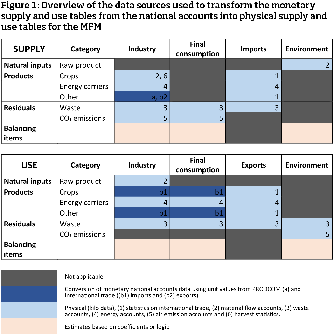
To compile the MFM, several Statistics Netherlands datasets need to be linked. More specifically, datasets on extracted and harvested goods, traded and produced goods, waste streams and emissions have to be combined. These datasets are mostly mandatory statistics based on surveys and data from national registers (e.g., trade registered by the Dutch customs authority). Figure 1 visualizes where the different datasets are applied to transform and extend the monetary supply and use tables from the national accounts into physical supply and use tables for the MFM. The main steps to develop the MFM are summarized in Table 1 below.
| Steps | Description | Datasets |
|---|---|---|
| Step 1 | Compile monetary supply and use tables (SUT) for products and services in basic prices. | National accounts supply and use tables |
| Step 2 | Convert monetary SUT of products to physical SUT. | Unit values derived from Prodcom, international trade data, agriculture statistics |
| Step 3 | Replace product flows in step 2 with available physical data. | Physical Energy Flow Accounts, international trade statistics, agriculture statistics |
| Step 4 | Add residual and natural resource material flows. | Waste statistics, material flow accounts, air emission accounts. |
| Step 5 | Add balancing items (e.g., O2 emissions for combustion processes, water uptake/loss products). | Conversion factors taken from MFA handbook (Eurostat, 2018) |
| Step 6 | Reconcile the supply and use (both per material and per sector) manually to a difference of max. 10%. | Not applicable |
| Step 7 | Reconcile the supply and use by automated modelling for the remaining differences. | Not applicable |
3.1 Compilation of monetary supply and use tables (SUT) in basic prices
Monetary supply and use tables are compiled annually at Statistics Netherlands as a subsystem of the national accounts according to internationally agreed standards (UN, 2009). The tables describing the supply and use of goods and services are published for 95 commodities in 81 sectors (CBS, 2021). For the MFM more detailed supply and use tables are used that are only available from Statistics Netherlands under strict confidentiality conditions. The supply table is available in basic prices. The use table is converted to basic prices too, by excluding margins, subsidies etcetera from the monetary value of products. In this way the monetary values become more consistent with the unit values applied for the conversion to kilos (see section 3.2).
As our aim is to estimate physical flows into, within and out of the economy, the second step entails changing the monetary supply and use tables to represent physical flows. In the national accounts, goods sent abroad for processing and returned – and vice versa – are not recorded as imports and exports of commodities but as imports or exports of processing services (Hiemstra, 2014). For example, the export of crude oil by British Petroleum to the Netherlands for refining and subsequent imports of the resulting petrol are recorded as the export of a refining service by the Netherlands in the national accounts if British Petroleum retains ownership of the crude oil/petrol. . In the MFM, we want to record these material flows as import of crude oil and export of petrol. To include such material flows, we add them to the monetary supply and use tables. Goods sent for processing and production abroad play a substantial part in the Dutch economy because the Netherlands is a small country with an open economy. In larger countries, these corrections might not be necessary if goods are not imported and exported for processing on a relevant scale.
3.2 Conversion of monetary SUT to physical SUT
Monetary supply and use tables are converted into physical supply and use tables using unit values, the price per kilo for a set of goods (dark blue cells of figure 1). As unit values may vary within one product group, they can differ on the supply side and the use side and per sector. Several sources are used to compile the set of unit values: production statistics (Prodcom), international trade statistics, and data on agriculture. We prioritized these sources based on quality as they may have unit value information on the same product group m. The agriculture data are considered to be the strongest source on the supply side, followed by Prodcom and lastly international trade statistics. Fewer sources are available on the use side; here unit values are derived solely from international trade statistics.
3.2.1 Deriving unit values from Prodcom data
The production statistics of manufactured goods, known as Prodcom (Eurostat, 2022b), provide information on the supply of approximately 4000 products by the mining and manufacturing sectors. They record both physical volumes (kg, m2, number of items, etc.) and financial values of sold products. To derive unit values, all physical volumes are converted to kilos using Eurostat conversion factors (Eurostat, 2021).
The advantage of Prodcom is that it provides data on heterogeneous goods for the various sectors. This means that different unit values are found depending on the sector supplying the product. The Prodcom data on kilos and values are based on a sample (excluding companies with fewer than 20 employees), so not all companies in a sector are represented. This does not affect the information on unit values much but simply adding up the data on kilos would result in an underestimation of the total production volume.
3.2.2 Deriving unit values from international trade data
The international trade dataset of Statistics Netherlands comprises imports and exports declared to the Dutch customs (extra EU trade) or reported by companies (intra EU trade). Within the EU, only trade above a certain value needs to be reported, Statistics Netherlands estimates the missing values. The international trade data contain detailed information on the type, value and weight of imported and exported goods.
The international trade data are used to derive unit values for most goods covered in the MFM (except for a few non-traded goods). These unit values are quantity-weighted averages of the different prices for which the products are purchased or sold. Some commodities are not recorded in kilo units (e.g., pieces or m2) and need to be converted to kilos first. For the supply tables, the unit values are used if no information is available in the agriculture statistics or in the Prodcom. Unit values of imported goods are used for the use side and unit values of exported goods for the supply side as some used goods are imported and some supplied goods are exported.
3.3 Improving and adding material flows
Only products with a monetary value are covered in the monetary SUTs. Therefore, sesiduals and natural resources are missing and need to be added. Physical data for some products are directly available from other sources (light blue cells in figure 1).
3.3.1 International trade
The international trade data also replace import and export figures from the monetary supply and use tables as the international trade data are considered to be more accurate. These figures overrule the imports and exports of the first estimates in the base table. Imports can be directly inserted in the supply table. Exports are divided between re-exports and exports from domestic production using the ratio of these variables from the monetary use table. Re-exports cannot exceed imports as by definition re-exports need to be imported first. Similarly, exports cannot exceed domestically produced products. These rules are taken into account throughout the entire process of compiling the MFM.
3.3.2 Energy carriers
Outcomes of the unit value estimations of energy carriers are replaced by physical data. Flows of energy carriers are derived from the Physical Energy Flow Accounts (PEFA), the SEEA energy accounts as implemented by Eurostat (2014; 2022c). Three adjustments are required to make this dataset compatible with the MFM.
First, the data in the PEFA are in tera joules (TJ) and need to be converted into million kilos. The conversion factors – taken from the MFA handbook (Eurostat, 2018) – differ per energy carrier. Some energy carriers, such as electricity, have no physical entity and are set to zero.
Second, PEFA categories of energy carriers need to be allocated to the energy carrier classification used in the MFM. Three extra energy carriers (goods) are added to the supply and use tables These are solid, liquid and gas biomass used for energy production.
Third, sectors in the PEFA need to be disaggregated to match the granularity of the sectors in the MFM. For example, ‘agriculture’ in the PEFA is divided into arable farming, horticulture, livestock farming, other agriculture, and agricultural services to match the MFM. To break these figures down correctly, multiple sources are used as a proxy for the division, among which the CO2 emission registration, the monetary tables of the national accounts, and the Energy balance sheet (CBS, 2022a). This results in data on the supply and use of energy carriers according to the categories of the MFM.
3.3.3 Additional data sources for agricultural yields
A separate source is available for unit values of agricultural goods such as grain, potatoes and flower bulbs. However, using these agricultural data alongside data from international trade still leaves a few cells empty. The missing unit values, for example for raw milk and cannabis, are found using websites.
3.3.4 Waste
Data on the production of waste are taken from the waste accounts (CBS, 2022b). Comparable data are collected by Eurostat for all EU countries. For these data too it is important that the granularity of the sectors (NACE codes) matches the level of detail in the MFM. This means more detail is needed than the Eurostat waste statistics provide. For the production of waste, NACE codes are broken down on the basis of monetary production figures from the national accounts and expert guesses.
On the use side, Eurostat publishes only the type of waste treatment. The allocation of waste use by NACE category is based on expert estimations. Recyclable waste is mostly used by the Materials recovery sector (NACE 38.3) for conversion to recovered products. Mineral waste, which accounts for a large part of the total produced waste, is mostly used in construction as foundation for roads and houses. Other waste is incinerated or, to a small extent, landfilled by the waste treatment sector.
CBS uses import and export figures on waste from the waste accounts. Companies are required to report trade of hazardous waste listed on the so-called red and orange lists. Trade of non-hazardous or ‘green’ waste is taken from trade statistics using a list of Combined Nomenclature waste codes compiled by Eurostat.
3.3.5 CO2 emissions
Data on CO2 emissions come from the annual air emissions accounts (Eurostat, 2022d). CO2 is supplied by sectors and used by the environment. Source data are available at aggregated sector level; allocation to the detailed MFM sectors is based on the ratio of the different emission relevant energy carriers, taking stationary and mobile emitters into account. Monetary supply and use tables are also used for the sector allocation. Data on CO2 emissions from non-combustion processes, such as chemical processes, are taken from the Pollutant Release and Transfer Register (for more information see http://www.emissieregistratie.nl).
Other type of emissions, CH4 and NOx, are not taken into account in the current MFM, as in weight terms these emissions are relatively small. However, for analytical purposes it might be interesting to add these emissions in future editions of the MFM.
3.3.6 Recovered products
In the Materials recovery sector (NACE 38.3), waste is collected and prepared for recycling. The physical (kilo) input of waste and the production of recycled materials are taken from Statistics Netherlands dataset Delivery and processing of waste at recycling companies (CBS, 2022c). The amount of recovered products and materials is estimated by subtracting produced waste from total collected waste. The use of recovered products produced by this sector and by other sectors is estimated using expert guesses. Further, we assumed that no products from this sector are imported or exported as no data are available.
3.3.7 Extraction
Many production processes use resources that are extracted from the environment. The MFM also classes crop harvesting by agriculture as a form of extraction. The environment is included as a separate sector in the MFM. Extraction is divided into crops, animal feed, wood, fish, salt, limestone, clay, sand, gravel, natural gas and crude oil. Data on extraction are taken from the Material Flow Accounts (MFA).Volumes of crops are allocated to the relevant agricultural sectors by the crop statistics (CBS, 2022d).
Some resources are extracted by more than one sector which makes the allocation in the use tables more difficult. For example, allocating salt extraction to the relevant sectors is done by looking at production data at company level. In the Netherlands, companies from the mineral and quarrying sector, and the chemical sector extract salt.
A number of checks are built in to ensure data validity: the supply of a certain good may not exceed extraction for example. The reason for this is that it is not possible to produce more of a product than goes into the production process. For example, the supply of agricultural goods cannot exceed the extraction of crops. Similarly, the supply of crude oil and natural gas should not exceed the extraction of crude oil and natural gas.
3.4 Adding balancing items
The physical supply and use tables need to be balanced and balancing items are added for material flows that are not recorded in the used statistics. The balancing of the physical supply and use tables follow the reconciliation rules of the monetary supply and use tables. Supply equals use for each good, as all materials supplied have to be used and input must equal output for each sector: industrial processes transform materials and products and either use or emit substances such as carbon dioxide, water, and oxygen. In order to balance sectors, balancing items are introduced (light pink cells in figure 1). The major balancing items are related to the uptake and emission of substances during the combustion of energy carriers, the gain or losses of water in products during the production process, and the service sectors like restaurants, that use materials but only produce services.
3.4.1 Combustion processes
For each sector a mass balance for energy combustion must apply: combustion of energy carrier plus O2 equals CO2 plus H20. Energy carriers and CO2 are already part of the MFM; O2 and H2O need to be introduced as balancing items.
The environment supplies O2 which is used by industry when combusting energy carriers. O2 intake can occur in two ways: by binding with carbon and by binding with hydrogen. To calculate O2 use during fuel combustion, the conversion factor of the O2 input per emission of CO2 is used. Similarly, the oxygen requirement for the oxidation of the hydrogen incorporated in the combusted material is determined. These two values of O2 (from CO2 and H2O) are added together.
H2O emissions occur during combustion processes in two ways. Hydrogen interacts with O2 during combustion processes, causing emission of H2O and the moisture content of the energy carrier evaporates. There are different conversion factors to estimate the O2 and H2O balancing items. The conversion factors are related to the emission-relevant energy carriers and the combustion-related CO2 emissions. We take the conversion factors from the MFA handbook (Eurostat, 2018).
3.4.2 Respiration (O2, H2O, CO2)
The respiration of humans and farm animals uses O2 and emits H2O and CO2 to the environment. Humans and domesticated animals are accounted for as part of the economy, and therefore the material flows are included in the balancing items. The number of farm animals are multiplied by their respective O2 use per year and allocated to the sector livestock farming. The human population in the Netherlands is also multiplied by the O2 use per person per year. This is allocated to the sector households. The data on the number of humans and livestock are compiled by Statistics Netherlands. Conversion factors are taken from the MFA handbook (Eurostat, 2018).
The same method is applied to calculate the CO2 and H2O supply of livestock and humans. The emission per animal and person of CO2 and H2O are multiplied by the number of animals and people and allocated to the supply of CO2 and H2O by livestock and households.
3.4.3 Nitrogen for the Haber-Bosch process
Nitrogen is taken from the air for the industrial production of ammonia (for fertilizer) in the Haber-Bosch process. The production of ammonia is multiplied by the conversion factor of ammonia to nitrogen. The nitrogen is used by the fertilizer industry and supplied by the environment. Data on the production of ammonia come from Prodcom. The factor to convert ammonia to the amount of nitrogen input is taken from the MFA handbook (Eurostat, 2018).
3.4.4 Water loss and addition
Bulk water is not part of the MFM. As a result, bulk water added during the production process causes an imbalance in sector input and output. For example, in the beverage industry, bulk water is added to produce beverages. Hence, the input (that does not include bulk water input) is much smaller than the output (that includes bulk water incorporated in the products).In addition, the water content (moisture) of products can change during the production process. For example, loss of water occurs while producing cheese from milk.
To determine the amount of water that is added or lost during the production process, we estimated the water content of all product groups based on literature. These water content coefficients are multiplied with the physical supply and use tables at the time the supply and use of goods are balanced by hand (differences below 10% remain). The result is a rough estimate of the water balance (loss or gain) for each sector. Due to the lack of data quality, this balance is only used as a reference figure while balancing the input and output of the sectors.
3.4.5 Service sector and other balancing items
The final balancing item added to the physical supply and use tables encompasses more than one kind of good used as input by the service sector. For example, construction sectors use a lot of materials such as sand and gravel. However, on the supply side there is barely any output because the national accounts record constructions such as buildings not as physical output but as a service. Services have no material component. The use surplus is therefore added to the supply of these sectors as a balancing item. In the agricultural sectors there is a lot of use of manure and fertilizers that is not part of the output, this is also accounted for in the balancing item on the supply side. A balancing item on the use side is also possible. For example, in a public economic sector like rail transport, waste produced by customers is not matched by the input of this sector.
3.5 Reconciling supply-use and input-output
The result of the methodology described in this chapter is a physical supply and use table. However, due to uncertainties of the different data sources and estimation methodologies, supply does not always equal use, even after inserting balancing items. The final step in completing the MFM is to reconcile the supply and use of goods and the input and output of sectors. Large differences are investigated and solved by hand and remaining smaller discrepancies are eliminated by modelling.
3.5.1 Manually
Any large differences are investigated and solved manually. Differences are considered to be large if they are more than 10% of the supply or larger than 1 billion kilos for goods or sectors. In order to be able to reduce balance differences, the source data need to be adjusted. Data considered to be least plausible are adjusted most. These are data which require the most assumptions to establish an estimate, often data on domestic use of products and waste. We present the balancing rules applied by Statistics Netherlands to create the MFM in Table 2 below.
| Part | Category | Flows that need to be in balance |
|---|---|---|
| Rows | Natural inputs | Extraction from environment = Domestic intermediate use industry |
| Products | Import + domestic production industry = Domestic intermediate and final use + export | |
| Residuals | Import + domestic production + final consumption domestic = Domestic intermediate and final use + exports + release to environment | |
| Columns | Industry | Input natural resources + products + residuals + balancing items = Output products + residuals + balancing items |
| Total PSUT | Total supply and total use | Supply = Use |
3.5.2 Modelling
The second step of data reconciliation is modelling to remove smaller discrepancies. We use a modified version of Stone’s method which is a generalized least-square method that “adjusts data in order to satisfy a set of linear constraints” (Eurostat, 2022e). The constraints make sure that a relation between two variables is fixed or remains within certain limits. The standard constraints are as follows. Supply equals use of goods and input equals output of sectors. Also, imports should equal or exceed re-exports as by definition re-exports need to be imported first. Similarly, domestic production cannot exceed exports. Additional constraints are inserted to create logical material flows. For example, the supply of processed meat may not exceed use of livestock and use of processed meat by abattoir. Additional calculation rules are explained in section 3.3.6 on extraction.
We slightly modified Stone’s method by introducing reliability weights in order to improve the figures (Bikker et al., 2012). The weights are devised to ensure that the figures deemed most reliable are modified least. Furthermore, the method allows exogenous variables, whose values must remain unmodified. For the MFM, the supply side is considered more reliable than the use side because more source data are available. Also data on international trade, energy carriers and extraction are considered to be robust. Data on the use of secondary materials by industry are considered the least reliable. The results of the model are always compared to the input. If it turns out that solutions found by the model are not plausible, further adjustments are made by hand to the original SUTs, after which the model is rerun.
3.6 Developing time series
Time series can be compiled by repeating the described methodology for every additional year However, repeating this method is not ideal for obtaining consistent time series if the underlying statistics change due to revisions. We divert to developments in time instead of actual data when consistencies over time are compromised because source data are revised. During a revision, new insights or definitions are implemented. In order to maintain a time-consistent MFM, we can no longer use the exact source data for an additional year. In this case, time series are compiled by applying the developments in time of the source data to the base year MFM. Data for a new year (t+2) are estimated by multiplying developments over time with the base year t. For example, if the source data from the emissions accounts report an increase in CO2 emissions of 6% between t and t+2 then the CO2 emissions of the MFM are increased by 6% to obtain the t+2 MFM.
Second, the methodology described in this chapter can be a time-intensive process that will not necessarily deliver the most consistent time series. This is the case for the MFM product categories that are estimated by converting monetary units to kilos by using unit values. Instead, for the supply and use of products the monetary volume development over time is used to estimate an additional year. By taking monetary developments in constant prices, volume changes due to price changes are ruled out. However, a disadvantage of this methodology is that quality improvements are also recorded as volume increments. For example, the recorded volume of a PC doubles when its performance doubles, even if its weight stays the same.
The longer the period between the base year and the years estimated by developments over time, the more the MFM figures deviate from the current state of affairs. Therefore, a periodic revision of the MFM is undertaken to implement changes in the source datasets and classifications, and to include new datasets if applicable. The MFM follows the revision strategy of the national accounts as closely as possible. For the national accounts, following EU policy, a revision takes place approximately every 5 to 6 years. During these revisions, new European guidelines are implemented, classifications are improved, new source data are applied and methodological adjustments are implemented.
After a revision, the MFM also needs to be revised retrospectively to achieve a consistent time series. When the MFM is revised, the revision is implemented for the base year of the most recent MFM. For this base year there are then two versions of the MFM: the revised and the unrevised version. The revised MFM is then extrapolated back in time to create a consistent, revised time series for earlier years. Developments back in time are derived from the unrevised MFM and applied to the revised base year.