Statistical combination of different types of chlorofyll-a measurements in the Dutch North Sea
About this publication
The report investigates the current method to combine different types of chlorofyll-a measurements in the Dutch North Sea and proposes an alternative approach.
Summary
The current approach uses weighted averages of in-situ and EO data based on confidence ratings, where the weight given to in-situ data can range from 10% to 50%, depending on the confidence in the data. However, significant discrepancies exist between the datasets, with in-situ measurements being sparse in both time and space. This can result in overrepresentation of in-situ data and leads to potential biases in the calculated growing season means.
The report proposes an alternative method that aggregates in-situ and EO data on a grid basis and imputes missing values before calculating growing season means. This approach aims to reduce the bias introduced by the low resolution of in-situ measurements. The report also introduces a new method for determining confidence ratings using the relative margin of error (MOE) to account for sample size variations across year–month–grid combinations. By setting thresholds for MOE, the report defines confidence ratings as ‘low,’ ‘moderate,’ or ‘high,’ providing a more systematic approach to assess the data quality.
Ultimately, too much weight may be given to the in-situ data in the current weighted approach, as this shows a moderate decrease in the chl-a trend between 1998 and 2020, while the alternative method produces a stable chl-a trend. The proposed changes offer a more accurate and balanced representation of chl-a levels, helping to improve the assessment of eutrophication in the OSPAR area.
1. Introduction
This report evaluates the current method of combining chl-a data by: 1) exploring the in-situ and EO datasets in both temporal and spatial contexts, 2) assessing how the weighting process influences growing season mean values, and 3) reviewing the criteria for determining the confidence rating. Thereafter, alternative methods for calculating chl-a growing season means and confidence ratings will be explored. The primary focus will be on the Dutch OSPAR assessment areas, mainly the Southern North Sea (SNS), but two smaller coastal areas, the Meuse plume (MPM) and the Rhine plume (RHPM), will also be discussed.
2. Data exploration
Both the EO and in-situ datasets were acquired through OSPAR, whereby the in-situ data can also downloaded through the ICES data portal. The chl-a indicator is used to address eutrophication, and thus only reflects concentrations in the upper 10 meters of the water column. While this depth limitation is inherent to the EO data, any in-situ measurements taken at greater depths are excluded from the analysis. Additionally, the indicator relies on growing season means, with the growing season, as defined by OSPAR, extending from March to September. The focus of this analysis is on these seven months, although algal blooms may occur outside this window, especially as climate change influences water temperatures in the North Sea1) 2). The analysis covers the period from 1998 to 2020, as both in-situ and EO data are available for these years.
2.1 In-situ data
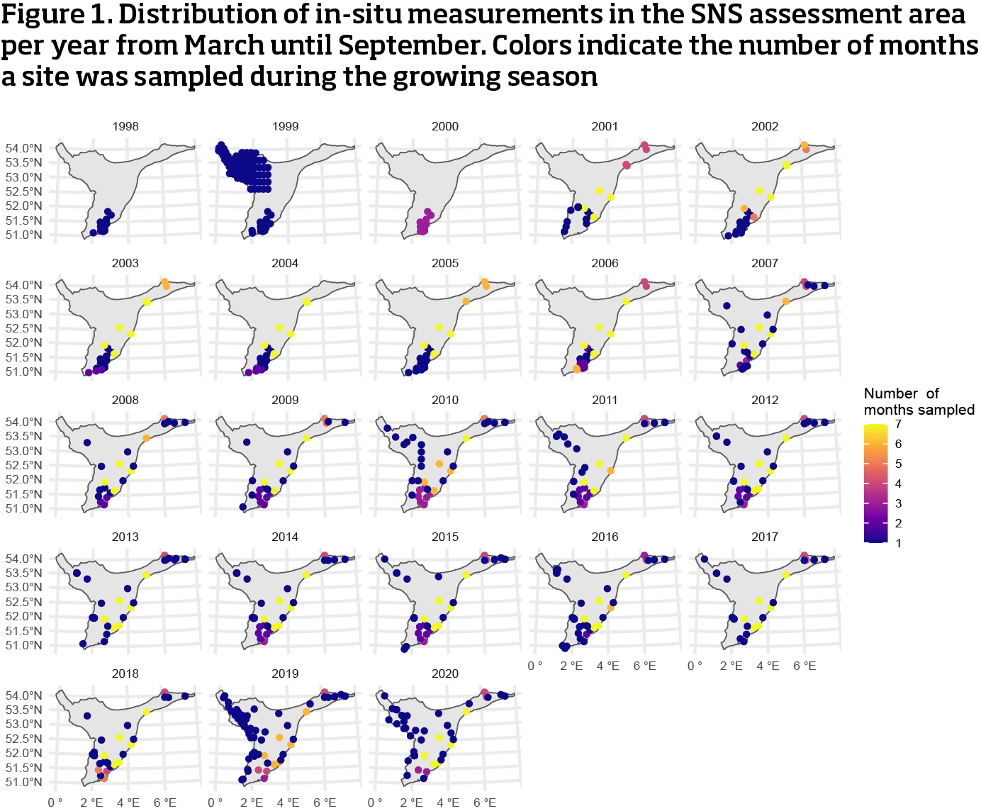
The number of in-situ measurements and chl-a concentrations in the Southern North Sea (SNS) assessment area are summarized in Table 1. The sample size fluctuated over the study period, with a peak in 2019, featuring approximately 131 samples during the growing season. The spatial distribution of these measurements is shown in Figure 1, which reveals that sampling sites are unevenly distributed, with a higher concentration of samples taken near the British, Belgian, and Dutch coasts. Only a few sites on the Dutch Continental Shelf were sampled throughout all months of the growing season, whereas most sites were sampled only during a single month (although not all in the same month, see distribution over months sampled per year in Table 1).
2019 was the most sampled year, and the development of quantile chl-a concentrations during that year’s growing season is depicted in Figure 2. Although no data is available for March, the results show elevated chl-a concentrations during the spring bloom, particularly near the Dutch coast. However, the sparse spatial distribution of samples makes it difficult to discern broader patterns across the entire SNS area.
| year | chl-a (mean) | chl-a (sd) | n | n months | n days |
|---|---|---|---|---|---|
| 1998 | 4,76 | 4,18 | 43 | 7 | 23 |
| 1999 | 18,90 | 15,83 | 128 | 4 | 15 |
| 2000 | 10,85 | 10,26 | 39 | 3 | 7 |
| 2001 | 6,54 | 6,70 | 78 | 7 | 37 |
| 2002 | 5,04 | 3,85 | 99 | 7 | 41 |
| 2003 | 6,80 | 8,59 | 108 | 7 | 43 |
| 2004 | 5,98 | 5,68 | 107 | 7 | 35 |
| 2005 | 4,80 | 5,08 | 103 | 7 | 40 |
| 2006 | 4,23 | 4,00 | 102 | 7 | 47 |
| 2007 | 4,91 | 5,82 | 80 | 7 | 39 |
| 2008 | 4,60 | 6,62 | 65 | 7 | 36 |
| 2009 | 3,38 | 4,63 | 94 | 7 | 46 |
| 2010 | 2,93 | 3,23 | 92 | 7 | 35 |
| 2011 | 4,17 | 4,93 | 103 | 7 | 46 |
| 2012 | 2,55 | 2,38 | 117 | 7 | 50 |
| 2013 | 2,51 | 3,17 | 106 | 7 | 46 |
| 2014 | 3,39 | 3,33 | 110 | 7 | 43 |
| 2015 | 4,25 | 4,11 | 107 | 7 | 47 |
| 2016 | 4,97 | 7,63 | 100 | 7 | 44 |
| 2017 | 4,15 | 6,37 | 90 | 7 | 43 |
| 2018 | 3,87 | 4,30 | 101 | 7 | 50 |
| 2019 | 2,75 | 4,66 | 131 | 6 | 56 |
| 2020 | 2,48 | 2,03 | 117 | 7 | 51 |
| 1) N is based on unique samples per site and timestamp, replicates are not considered. | |||||

2.2 Earth Observation data
EO data is extremely well sampled throughout the SNS assessment area (Table 2), with millions of measurements that span the entire duration of the growing season. All months, and almost all days, are sampled during each year in contrast to the in-situ data (Table 1). For more background on the acquisition of EO data, see Van der Zande et al. (2019)3) and Lavigne et al. (2021)4).
| year | chl-a (mean) | chl-a (sd) | n | n months | n days |
|---|---|---|---|---|---|
| 1998 | 3,19 | 3,08 | 2072362 | 7 | 188 |
| 1999 | 3,73 | 4,37 | 3294312 | 7 | 202 |
| 2000 | 2,43 | 2,14 | 2733508 | 7 | 190 |
| 2001 | 4,21 | 4,87 | 3330415 | 7 | 181 |
| 2002 | 2,79 | 1,89 | 4121014 | 7 | 196 |
| 2003 | 3,54 | 3,27 | 6032644 | 7 | 204 |
| 2004 | 2,98 | 2,40 | 5013950 | 7 | 203 |
| 2005 | 2,92 | 2,48 | 4641851 | 7 | 197 |
| 2006 | 2,77 | 2,28 | 5533996 | 7 | 195 |
| 2007 | 3,48 | 3,45 | 5126752 | 7 | 204 |
| 2008 | 3,71 | 3,51 | 4928548 | 7 | 206 |
| 2009 | 2,85 | 3,06 | 5506865 | 7 | 209 |
| 2010 | 3,43 | 3,41 | 5109299 | 7 | 200 |
| 2011 | 3,13 | 3,11 | 5019536 | 7 | 197 |
| 2012 | 2,60 | 2,56 | 5259718 | 7 | 201 |
| 2013 | 3,59 | 3,69 | 5757591 | 7 | 195 |
| 2014 | 3,04 | 3,43 | 5187452 | 7 | 203 |
| 2015 | 3,03 | 3,37 | 5619866 | 7 | 205 |
| 2016 | 2,90 | 2,94 | 6327410 | 7 | 207 |
| 2017 | 2,63 | 2,54 | 5882981 | 7 | 208 |
| 2018 | 2,72 | 2,59 | 6198899 | 7 | 205 |
| 2019 | 2,73 | 2,88 | 5942578 | 7 | 208 |
| 2020 | 3,00 | 2,52 | 6692037 | 7 | 210 |
Table 2 highlights the temporal coverage of the Earth Observation (EO) data, while Figure 3 presents the spatial distribution of this data for the year 2019. To appropriately visualize the data, chl-a concentrations were aggregated to a 5x5 km grid (the original resolution of the EO data being 1x1 km). These aggregated values were then categorized into quantiles. The results demonstrate that the EO data effectively captures both spatial and temporal patterns of chl-a concentrations throughout the growing season. Notably, higher concentrations are observed during early phytoplankton blooms from March to May, with levels being generally elevated near the coast.
In the later years of the monitoring period, the EO data provides excellent coverage of the SNS area. However, coverage was less comprehensive in the earlier years (see differences in n Table 2; and Figure 4), with some months showing gaps in 5x5 km grid data. Despite these early gaps, the EO data coverage of the SNS area remains nearly complete.


2.3 Conclusion data exploration
Large differences exist between the spatial and temporal distribution of the in-situ and EO datasets, with the two datasets not being directly comparable, as illustrated in Table 3. The number of in-situ samples is substantially smaller than that of the EO data, both in terms of temporal coverage and spatial distribution. In-situ data is not representative of the entire SNS assessment area, and in many years, there are gaps where not all months of the growing season were sampled.
Given these discrepancies, a strong recommendation is to treat in-situ samples as individual data points alongside the EO data. Aggregating both datasets before calculating growing season averages may provide a more accurate representation of the overall conditions. If and how the current weighting method may introduce biases is explored in the next chapter.
| year | n EO | n in-situ | n total | % in-situ | % EO |
|---|---|---|---|---|---|
| 1998 | 2072362 | 43 | 2072405 | 0,0021 | 99,9979 |
| 1999 | 3294312 | 128 | 3294440 | 0,0039 | 99,9961 |
| 2000 | 2733508 | 39 | 2733547 | 0,0014 | 99,9986 |
| 2001 | 3330415 | 78 | 3330493 | 0,0023 | 99,9977 |
| 2002 | 4121014 | 99 | 4121113 | 0,0024 | 99,9976 |
| 2003 | 6032644 | 108 | 6032752 | 0,0018 | 99,9982 |
| 2004 | 5013950 | 107 | 5014057 | 0,0021 | 99,9979 |
| 2005 | 4641851 | 103 | 4641954 | 0,0022 | 99,9978 |
| 2006 | 5533996 | 102 | 5534098 | 0,0018 | 99,9982 |
| 2007 | 5126752 | 80 | 5126832 | 0,0016 | 99,9984 |
| 2008 | 4928548 | 65 | 4928613 | 0,0013 | 99,9987 |
| 2009 | 5506865 | 94 | 5506959 | 0,0017 | 99,9983 |
| 2010 | 5109299 | 92 | 5109391 | 0,0018 | 99,9982 |
| 2011 | 5019536 | 103 | 5019639 | 0,0021 | 99,9979 |
| 2012 | 5259718 | 117 | 5259835 | 0,0022 | 99,9978 |
| 2013 | 5757591 | 106 | 5757697 | 0,0018 | 99,9982 |
| 2014 | 5187452 | 110 | 5187562 | 0,0021 | 99,9979 |
| 2015 | 5619866 | 107 | 5619973 | 0,0019 | 99,9981 |
| 2016 | 6327410 | 100 | 6327510 | 0,0016 | 99,9984 |
| 2017 | 5882981 | 90 | 5883071 | 0,0015 | 99,9985 |
| 2018 | 6198899 | 101 | 6199000 | 0,0016 | 99,9984 |
| 2019 | 5942578 | 131 | 5942709 | 0,0022 | 99,9978 |
| 2020 | 6692037 | 117 | 6692154 | 0,0017 | 99,9983 |
2) Tinker, J., Lowe, J., Pardaens, A., Holt, J., & Barciela, R. (2016). Uncertainty in climate projections for the 21st century northwest European shelf seas. Progress in Oceanography, 148, 56–73.
3) Van der Zande, D., Lavigne H., Blauw A., Prins T., Desmit X., Eleveld M., Gohin F., Pardo S., Tilstone G., Cardoso Dos Santos J., Coherence in Assessment Framework of Chlorophyll A and Nutrients as Part of the EU Project ‘Joint Monitoring Programme of the Eutrophication of the North Sea With Satellite Data’ (Ref: DG ENV/MSFD Second Cycle/2016) (2019). Activity 2 Report (106 pp)
4) Lavigne H., Van der Zande D., Ruddick K., Cardoso Dos Santos J., Gohin F., Brotas V., Kratzer S., Quality-control tests for OC4, OC5 and NIR-red satellite chlorophyll-a algorithms applied to coastal waters (2021). Remote Sensing of Environment 255: 112237.
3. Current method
3.1 Confidence rating
In the current approach for combining in-situ and EO data to determine chl-a growing season means, the means of both datasets are first calculated separately. A weighted average is then computed based on the confidence rating of each dataset, following criteria that consider both spatial and temporal confidence aspects. These criteria are detailed in Annex 13 of the OSPAR eutrophication status assessment procedure . If the in-situ data has high confidence, a weighting of 50:50 (in-situ/EO) is applied; for moderate confidence, the ratio is 30:70 (in-situ/EO), and for low confidence, it shifts to 10:90 (in-situ/EO).
Even when the confidence of the in-situ data is low, assigning it a 10% weight remains significant, especially considering the large discrepancy in the representativeness of in-situ versus EO data across the growing season (see chapter 2), with the in-situ data representing at best 0,0039% of all combined measurements taken in 1999.
To demonstrate the impact of different weightings on growing season means, Figure 5 illustrates all weighting scenarios considered in the present study, including the individual means of in-situ and EO data, as well as the weighting used in OSPAR. With the exception of 2002, a 50:50 weighting was applied in all years. However, these weighting factors were determined somewhat subjectively. There is no statistical backing for boundaries at which the confidence classes and the corresponding weights are set5), but as a result, high in-situ values can disproportionately affect the calculated growing season means.
Since in-situ data is collected sporadically compared to EO data, there is a possibility that extremely high chl-a concentrations may be captured due to the timing of in-situ sampling during periods of high phytoplankton density, such as algal blooms, and/or the higher variation in sample sites. For instance, in 1999, the area around the British shore was extensively sampled in contrast to other years (Figure 1), and samples were only taken during four months of the growing season (Table 1).
An argument often cited to support the use of in-situ data is the claimed higher precision of chl-a measurements compared to EO data. However, comparisons between in-situ and EO chl-a measurements in the Baltic Sea reveal that the uncertainties associated with both methods fall within the same range6). Furthermore, these comparisons were made using chl-a products derived from MERIS and OLCI satellites. In contrast, the Sentinel satellites, which have been in use since 2016 and incorporate the JMP EUNOSAT quality control, offer even greater precision.

3.2 Conclusion current method
The current method of integrating in-situ and EO data is highly sensitive to temporal and spatial biases in the in-situ measurements. As a result, the elevated chl-a concentrations observed at the start of the time series are likely to be artifacts of the methodology. Investigating alternative approaches for data integration could provide more robust results and is recommended.
6) Kratzer, S., Harvey, E.T., Canuti, E., International Intercomparison of In Situ Chlorophyll-a Measurements for Data Quality Assurance of the Swedish Monitoring Program (2022). Frontiers in Remote Sensing 3 2673-6187.
4. New method – data aggregation
In this chapter, we present an alternative approach for determining chl-a growing season means and their associated confidence ratings, addressing the imbalances between in-situ and EO measurements. This method considers the variation in spatio-temporal distribution during the growing season and accounts for missing data.
Given the discrepancies between in-situ and EO measurements, an aggregation of these datasets is recommended before performing any further calculations, as the weighting method currently overemphasizes the influence of in-situ samples (chapter 3). Moreover, variations in the spatio-temporal distribution of both EO and in-situ measurements necessitate aggregation prior to calculating growing season means (Figure 6). Before combining in-situ and EO data into a single growing season mean, separate means are calculated. However, these means are derived by simply averaging the data over the entire growing season without accounting for temporal and spatial variations (Figure 6). In certain months and regions, more measurements may be available due to favorable weather conditions, leading to overrepresentation of specific areas or periods (for both EO and in-situ data). This approach can result in a skewed representation of chl-a concentrations, particularly as coastal regions and certain months tend to exhibit higher concentrations (Figure 3 and Figure 4).

Our approach will thus treat in-situ measurements as individual data points alongside EO data, aggregating both on a year-month-grid basis before proceeding with analyses. The focus will be on 1) determining the optimal grid size for aggregation, 2) imputing missing values, 3) calculating growing season means, and 4) introducing a new method for confidence ratings.
4.1 Optimal grid size
As stated above, a grid-based approach can effectively cope with temporal and spatial variation in chl-a measurements. The optimal grid size may be determined by identifying the sample size at which the variation in measurements becomes less pronounced. Figure 7 illustrates this relationship by plotting the standard deviation against sample size for four random 10x10 km grids across different months in 2008. While the sample size at which the standard deviation stabilizes varies between grids, a sample size of approximately 100 appears to provide a reliable estimate of chl-a. When dividing the SNS into 5x5 km grids, 12% of the grids have fewer than 100 samples, whereas only 6% of grids fall below this threshold when using a 10x10 km grid.

Grids are assigned to assessment areas based on their initial shapes, and may thus overlap between two neighboring areas. However, only the corresponding datapoints that lie within the initial shape of the assessment area are considered for further calculations. Dividing the study area into grids introduces edge effects, particularly where only part of the geographical area falls within the boundary of a grid cell (Figure 6). This results in smaller sample sizes at the edges. While in a large area like the SNS, these effects do not significantly impact the overall confidence rating, they become more pronounced in smaller coastal OSPAR assessment areas, where edge areas make up a relatively larger portion (Figure 8). Over the entire study period, using a 5x5 km grid results in 46% and 40% of grids containing fewer than 100 samples in RHPM and MPM, respectively. In contrast, using a larger 10x10 km grid reduces these percentages to 28% and 25%, thereby improving the confidence rating. Also in later years, with higher resolution EO data, edge effects are more prominent in smaller assessment areas.

Another important consideration when determining grid size is its impact on the mean growing season values. Utilizing a smaller grid size helps minimize the loss of resolution during the aggregation process. Table 4 illustrates the differences in growing season means for various grid sizes. Across the whole study period, the mean growing season difference between the 5x5 and 10x10 grids is 0.05 μg L-1 chl-a, while the difference between the 5x5 and 25x25 grids is 0.2 μg L-1 chl-a. Although increasing the sample size up to approximately 250 samples can improve the reliability of chl-a estimates, selecting a grid size that is too coarse beyond this threshold may lead to a significant loss of resolution. Do note that mean values in the coarser grid size are consistently higher than the smaller grid size, due to the relatively higher contribution of grids with higher mean chl-a values (high chl-a concentrations can sometimes be 100 times higher than background concentrations, which impacts mean concentrations).
A 10x10 km grid may represent the optimal choice, as it offers a sufficient sample size to provide reliable chl-a estimates on a year – month – grid basis while minimizing edge effects and resolution losses. Consequently, further analyses will be conducted using this grid size.
| year | chl-a (mean 5x5) | chl-a (mean 10x10) | chl-a (mean 25x25) |
|---|---|---|---|
| 1998 | 3,08 | 3,12 | 3,15 |
| 1999 | 3,78 | 3,84 | 3,92 |
| 2000 | 2,66 | 2,71 | 2,75 |
| 2001 | 4,00 | 4,05 | 4,15 |
| 2002 | 3,00 | 3,05 | 3,18 |
| 2003 | 3,63 | 3,67 | 3,86 |
| 2004 | 3,06 | 3,11 | 3,22 |
| 2005 | 3,06 | 3,11 | 3,23 |
| 2006 | 3,09 | 3,14 | 3,26 |
| 2007 | 3,50 | 3,57 | 3,78 |
| 2008 | 3,76 | 3,82 | 3,98 |
| 2009 | 3,02 | 3,07 | 3,26 |
| 2010 | 3,39 | 3,44 | 3,66 |
| 2011 | 3,21 | 3,26 | 3,44 |
| 2012 | 2,82 | 2,88 | 3,08 |
| 2013 | 3,94 | 3,98 | 4,13 |
| 2014 | 3,27 | 3,33 | 3,51 |
| 2015 | 3,24 | 3,31 | 3,47 |
| 2016 | 3,18 | 3,23 | 3,44 |
| 2017 | 2,71 | 2,76 | 2,87 |
| 2018 | 3,03 | 3,08 | 3,26 |
| 2019 | 2,76 | 2,80 | 2,94 |
| 2020 | 2,91 | 2,96 | 3,09 |
4.2 Missing values
Particularly in the beginning of the study period, certain year–month–grid combinations are missing (Table 5; SNS area). Since only a small portion of the data is missing, the remaining data can be used to impute these missing values. One approach is the use of a random forest algorithm, implemented through the R package missForest7). This method preserves the relationships and distributions of the observed data, is resistant to overfitting, and is capable of handling high-dimensional data.
The accuracy of the imputation using missForest was evaluated using the Normalized Root Mean Square Error (NRMSE) metric. An exceptionally low NRMSE of 3.4 × 10⁻⁷ was obtained, indicating that the imputed values closely align with the observed data and demonstrate strong model performance with minimal prediction error.
Given the small proportion of missing data, the impact of imputing these values on the overall mean per growing season is minimal (Table 6), with a maximum difference of only 0.02 μg L-1 chl-a in 1998. For the SNS area, imputing missing values may therefore not be necessary, as the effect on the overall mean is negligible, and the process introduces an additional step in data handling. However, this may not be the case for other OSPAR assessment areas, where imputing missing values may be more relevant for a comprehensive analysis. For instance, the proportion of missing year–month–grid data in the MPM and RHPM regions combined varies from 11 to 17% between 1998 and 2001 (Table 5; MPM & RHPM), although missing values do not pose an issue in later years.
| SNS | MPM & RHPM | |||
|---|---|---|---|---|
| year | n missing | n measured | n missing | n measured |
| 1998 | 102 | 4917 | 112 | 623 |
| 1999 | 37 | 4982 | 80 | 655 |
| 2000 | 71 | 4948 | 128 | 607 |
| 2001 | 74 | 4945 | 112 | 623 |
| 2002 | 16 | 5003 | 22 | 713 |
| 2003 | 0 | 5019 | 0 | 735 |
| 2004 | 0 | 5019 | 0 | 735 |
| 2005 | 1 | 5018 | 2 | 733 |
| 2006 | 0 | 5019 | 0 | 735 |
| 2007 | 0 | 5019 | 0 | 735 |
| 2008 | 3 | 5016 | 0 | 735 |
| 2009 | 0 | 5019 | 0 | 735 |
| 2010 | 0 | 5019 | 0 | 735 |
| 2011 | 3 | 5016 | 0 | 735 |
| 2012 | 0 | 5019 | 0 | 735 |
| 2013 | 2 | 5017 | 4 | 731 |
| 2014 | 0 | 5019 | 0 | 735 |
| 2015 | 0 | 5019 | 0 | 735 |
| 2016 | 0 | 5019 | 2 | 733 |
| 2017 | 0 | 5019 | 0 | 735 |
| 2018 | 0 | 5019 | 0 | 735 |
| 2019 | 1 | 5018 | 0 | 735 |
| 2020 | 0 | 5019 | 0 | 735 |
| year | chl-a (mean with imputations) | chl-a (mean only observations) | difference |
|---|---|---|---|
| 1998 | 3,13 | 3,12 | 0,0187 |
| 1999 | 3,85 | 3,84 | 0,0096 |
| 2000 | 2,73 | 2,71 | 0,0229 |
| 2001 | 4,05 | 4,05 | 0,0047 |
| 2002 | 3,06 | 3,05 | 0,0092 |
| 2003 | 3,67 | 3,67 | 0 |
| 2004 | 3,11 | 3,11 | 0 |
| 2005 | 3,11 | 3,11 | 0,0006 |
| 2006 | 3,14 | 3,14 | 0 |
| 2007 | 3,57 | 3,57 | 0 |
| 2008 | 3,82 | 3,82 | 0,0002 |
| 2009 | 3,08 | 3,08 | 0 |
| 2010 | 3,44 | 3,44 | 0 |
| 2011 | 3,26 | 3,26 | 0,0009 |
| 2012 | 2,88 | 2,88 | 0 |
| 2013 | 3,98 | 3,98 | 0,0006 |
| 2014 | 3,33 | 3,33 | 0 |
| 2015 | 3,31 | 3,31 | 0 |
| 2016 | 3,23 | 3,23 | 0 |
| 2017 | 2,76 | 2,76 | 0 |
| 2018 | 3,08 | 3,08 | 0 |
| 2019 | 2,80 | 2,80 | 0,0002 |
| 2020 | 2,96 | 2,96 | 0 |
4.3 Trends
To illustrate the effect of the new method to calculate chl-a growing season means as compared to the current weighting method, we calculated the trend over the years using TrendSpotter8). This approach detects and estimates non-linear trends in environmental time series, and calculates standard errors and concomitant confidence intervals based on the Kalman-filter framework. In addition, the difference between the modelled trend value (the red line in figure 10) in each year and the model value in the last year is calculated. This enables the assessment of multiplicative trends (the percentage yearly change) and confidence intervals9), which are the base for a classification in increasing, stable, decreasing or uncertain trends (Figure 9).
By giving the in-situ data 50% weight in most years, the high in-situ chl-a concentrations, especially at the start of the monitoring period, influence the overall mean and this results in an overall moderate decrease in chl-a between 1998 and 2020, while the trend is stable in the new method (Figure 10). In the new method, in-situ and EO data were first aggregated on the 10x10 km scale, and missing values were imputed (Table 6).


4.4 Confidence rating – new method
In the current COMPEAT assessment the confidence rating per OSPAR assessment area for the chl-a measurements for both in-situ and EO data depends on the same criteria in Annex 13 of the OSPAR eutrophication status procedure6. These criteria, originally based on in-situ measurements, assign weights of 50%, 30%, or 10% to the in-situ data, though these weights lack a formal statistical foundation. Here, we propose a method that assigns a confidence rating to each year–month–grid combination based on sample size, which can then be aggregated to derive an overall confidence rating for the chl-a growing season mean each year.
To determine the confidence classes with sample size for each OSPAR assessment area, we will use the relative margin of error (MOE). The MOE quantifies the amount of random sampling error and represents the radius (= half) of the confidence interval. A 95% confidence interval reflects the 95% likelihood that the true value lies within that interval and is bounded by one MOE below and one MOE above the estimated mean. By using the relative MOE (the MOE divided by the mean), we adjust for variations in mean chl-a values across year–month–grid combinations. As shown in Figure 11, the relative MOE decreases as the sample size increases.

The sample size at which the relative MOE falls below a specified threshold can be used to define the boundaries for ‘low’, ‘moderate,’ or ‘high’ confidence ratings. The choice of relative MOE thresholds for confidence ratings depends on the acceptable error range. Given the typically large sample sizes per year–month–grid combination, we suggest to set the ‘moderate confidence’ boundary at a relative MOE of 0.1 and the ‘high confidence’ boundary at 0.05, corresponding to an error range of 10% and 5% respectively. For example, in Figure 11, the relative MOE drops below a threshold of 0.1 at a sample size of approximately 50 for grid 668 in July 2008. At this sample size, the mean chl-a value for that specific year–month–grid combination has a 10% error range (= 0.1 on the Y-axis) with 95% confidence. Likewise, the relative MOE for grid 453 in June drops below 0.05 at a sample size of about 200, so the error range for this year–month–grid combination is 5% at that sample size.
Despite small differences between year–month–grid combinations, the relative MOE curves in Figure 11 show a comparable pattern. Therefore, general sample size thresholds for each year–month–grid combination in the entire SNS area were assessed. We randomly sampled 100 grids for each year–month combination with a sample size greater than 100. For each grid, chl-a measurements were sampled up to a size of 800, with replacement, and the relative MOE was calculated (as shown in Figure 11). An exponentially decaying function was then fitted to each year–month–grid combination:
relative MOE \(= a \times \text{sample size}^b\)
with the nonlinear least squares (nls) function in R, where the a and b parameters were estimated by the model. Based on the fitted values, the sample size corresponding to the 0.1 and 0.05 MOE thresholds was determined for each year–month–grid. The means of these sample sizes serve as the overall confidence class boundaries for the SNS area. A threshold of 0.1 corresponds to a sample size of approximately 50 (‘moderate confidence boundary’), and a threshold of 0.05 corresponds to a sample size of around 200 (‘high confidence boundary’).
Per year–month–grid confidence classes can thus be assigned based on sample size. For subsequent aggregation per year–grid or per year classes were assigned numerical values of 1 (‘low confidence’), 2 (‘moderate confidence’) or 3 (‘high confidence’), where the overall mean determines the confidence rating. A score smaller than 1.5 represents a low confidence rating, between 1.5 and 2.5 a moderate confidence rating and a score higher than 2.5 a high confidence rating, as shown on the map in Figure 12. Results aggregated per year are shown in Table 7, including numerical scores. Some edge effects are present, as discussed in chapter 4.1, but these do not significantly affect the confidence rating.
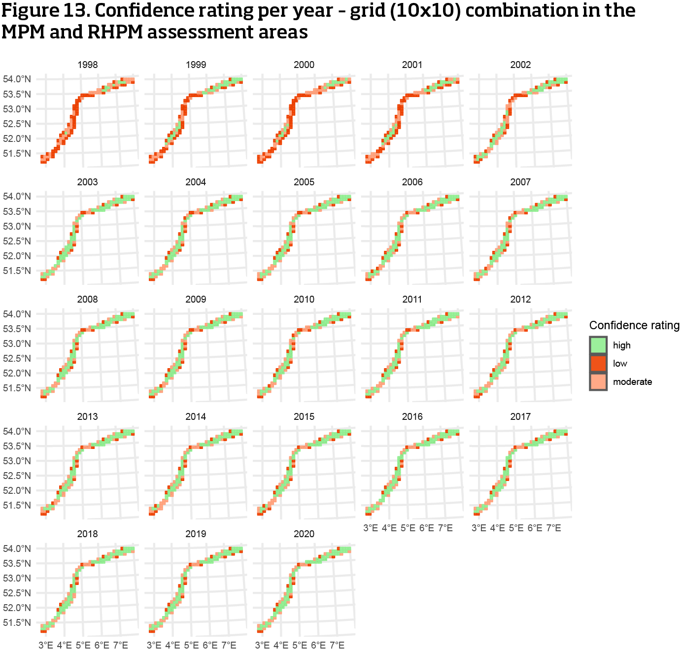
The same method can be used for the MPM and RHPM coastal areas, where we first determined the MOE thresholds based on chl-a measurements and sample sizes. As a result of the higher variation in chl-a concentrations closer to shore, the threshold of 0.1 corresponds to a sample size of approximately 60 (‘moderate boundary’), and the threshold of 0.05 corresponds to a sample size of around 260 (‘high boundary’). Consequently, confidence rating is on average lower than in the SNS area (Figure 13 and Table 7).

| SNS | MPM & RHPM | ||||
|---|---|---|---|---|---|
| year | confidence score | confidence class | year | confidence score | confidence class |
| 1998 | 2,58 | high | 1998 | 1,60 | moderate |
| 1999 | 2,81 | high | 1999 | 1,85 | moderate |
| 2000 | 2,67 | high | 2000 | 1,68 | moderate |
| 2001 | 2,68 | high | 2001 | 1,81 | moderate |
| 2002 | 2,85 | high | 2002 | 2,12 | moderate |
| 2003 | 2,90 | high | 2003 | 2,45 | moderate |
| 2004 | 2,89 | high | 2004 | 2,37 | moderate |
| 2005 | 2,85 | high | 2005 | 2,31 | moderate |
| 2006 | 2,89 | high | 2006 | 2,38 | moderate |
| 2007 | 2,88 | high | 2007 | 2,35 | moderate |
| 2008 | 2,88 | high | 2008 | 2,36 | moderate |
| 2009 | 2,89 | high | 2009 | 2,41 | moderate |
| 2010 | 2,88 | high | 2010 | 2,35 | moderate |
| 2011 | 2,88 | high | 2011 | 2,36 | moderate |
| 2012 | 2,89 | high | 2012 | 2,39 | moderate |
| 2013 | 2,89 | high | 2013 | 2,40 | moderate |
| 2014 | 2,89 | high | 2014 | 2,37 | moderate |
| 2015 | 2,89 | high | 2015 | 2,39 | moderate |
| 2016 | 2,90 | high | 2016 | 2,48 | moderate |
| 2017 | 2,90 | high | 2017 | 2,46 | moderate |
| 2018 | 2,90 | high | 2018 | 2,50 | moderate |
| 2019 | 2,90 | high | 2019 | 2,45 | moderate |
| 2020 | 2,90 | high | 2020 | 2,53 | high |
4.5 Conclusions new method
We propose to first aggregate chl-a data of different methods on a 10x10 km grid scale. This approach allows for adjustments based on variations in sampling effort, while its impact on the overall yearly means is expected to be minimal. Additionally, we recommend a new, more objective method for assigning confidence ratings, where boundaries can be set based on acceptable error range.
8) Visser, H., Estimation and detection of flexible trends (2004). Atmospheric Environment 38:4135–4145
9) Soldaat, L., Visser, H., Van Roomen, M., Van Strien, A., (2007). Smoothing and trend detection in waterbird monitoring data using structural time-series analysis and the Kalman filter. J. Ornithol. 148 (2): 351–357.
5. Discussion
The assessment of chl-a levels is essential for understanding eutrophication in the OSPAR maritime area, and the current method of combining in-situ and Earth Observation (EO) data provides a valuable, albeit imperfect, approach to estimating chl-a concentrations. One key issue identified in this analysis is the disparity between the temporal and spatial distributions of the in-situ and EO datasets, with in-situ samples being far less representative for the entire assessment area. Despite this, the current methodology often assigns significant weight to in-situ data, even when its confidence rating is low. This overemphasis may lead to inflated growing season means in years where in-situ measurements are coincidentally biased towards high chl a values, such as algal blooms.
Our findings suggest that the current weighting approach, especially the 50:50 weighting used in most years, can introduce bias into the overall chl-a means. In years with high in-situ chl-a concentrations, particularly during the early monitoring period, this bias leads to a moderate downward trend in chl-a levels from 1998 to 2020. However, when applying the alternative method presented in this report—where in-situ and EO data are aggregated on a year–month–grid basis—the trend is stable over time. This indicates that too much weight is given to the sporadic high in-situ values in the current method, and that the alternative method may provide a more accurate reflection of overall eutrophication trends. It is noteworthy that this new approach significantly diminishes the influence of in-situ measurements in monitoring eutrophication, bringing it close to negligible levels.
Furthermore, the introduction of confidence ratings based on the relative margin of error (MOE) offers a robust framework for assessing the reliability of chl-a estimates. By linking confidence ratings to sample sizes, we have provided a method for determining ‘low,’ ‘moderate,’ and ‘high’ confidence levels across different OSPAR assessment areas. The confidence rating thresholds for these classes can be determined per OSPAR area. For instance, the coastal the Meuse and Rhine plumes have higher sample size thresholds than the Southern North Sea due to increased variability in chl-a concentrations closer to shore. However, differences in confidence rating thresholds between these assessment areas were relatively small, meaning these thresholds may be determined more generally for the entire OSPAR maritime area. They could be established conservatively, including more grids with higher chl-a variation, but this would require data from more assessment areas. As an example the MOE threshold for a high rating was set to 0.05, and the threshold for a moderate rating to 0.1 in this report, however these thresholds can be adjusted to the acceptable error range. Moreover, data was aggregated on a 10x10 km scale, as it provided the sufficient sample size for reliable chl-a estimates, while minimizing edge effects and resolution losses. Optimal grid size should also be determined for other assessment areas.
In conclusion, the revised approach reduces the bias introduced by low resolution in-situ measurements and provides a clearer picture of eutrophication trends, supporting more informed decision-making for environmental management in the OSPAR maritime area.